FSRmdrrs
FSRmdrrs performs random start monitoring of minimum deletion residual
Description
Examples
 Random start for a simulated example with two small groups.
Random start for a simulated example with two small groups.An example with simulated data with regression lines with roughly the same number of observations.
close all
rng('default')
rng(2);
b1=[1 1];
b2=[1 2.6];
n1=40;
n2=50;
s1=0.1;
s2=0.1;
X1=rand(n1,1);
X2=rand(n2,1);
y1=randn(n1,1)*s1+b1(1)+b1(2)*X1;
y2=randn(n2,1)*s2+b2(1)+b2(2)*X2;
hold('on')
plot(X1,y1,'o');
plot(X2,y2,'o');
title('Two simulated regression lines')
y=[y1;y2];
X=[X1;X2];
figure
% parfor of Parallel Computing Toolbox is used (if present in current computer)
% and pool is not cleaned after % the execution of the random starts
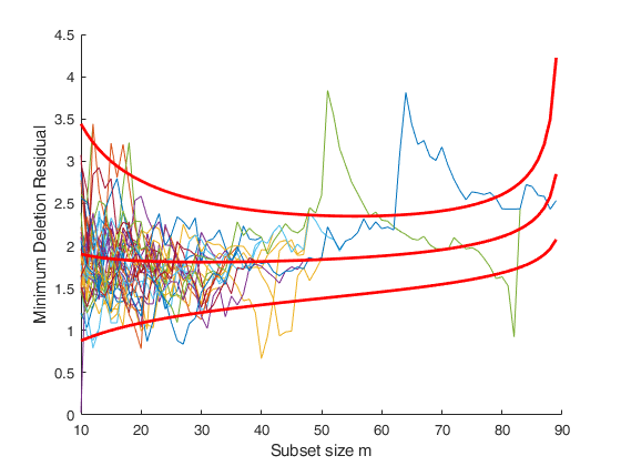
[out]=FSRmdrrs(y,X,'constr','','nsimul',50,'init',10,'plots',1,'cleanpool',false);
disp('The two peaks in the trajectories of minimum deletion residual (mdr).')
disp('clearly show the presence of two groups.')
disp('The decrease after the peak in the trajectories of mdr is due to the masking effect.')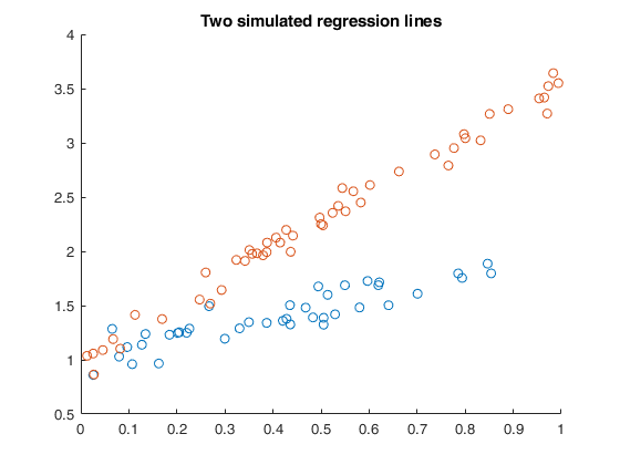
Random start for a simulated example with two groups.
Same example as before but now the values of n1 and n2 (size of the two groups) have been increased. In this case it is possible to see that there are two trajectories of minimum deletion residual which go outside the envelopes in the central part of the search.
% In this case the two groups have roughly the same size (n1=140 and n2=150)
close all
rng(2);
b1=[1 1];
b2=[1 2.6];
n1=140;
n2=150;
s1=0.1;
s2=0.1;
X1=rand(n1,1);
X2=rand(n2,1);
y1=randn(n1,1)*s1+b1(1)+b1(2)*X1;
y2=randn(n2,1)*s2+b2(1)+b2(2)*X2;
hold('on')
plot(X1,y1,'o');
plot(X2,y2,'o');
title('Two simulated regression lines')
y=[y1;y2];
X=[X1;X2];
figure
% parfor of Parallel Computing Toolbox is used (if present in current
% computer) and pool is not cleaned after
% the execution of the random starts
% The number of workers which is used is the one specified
% in the local/current profile
[out]=FSRmdrrs(y,X,'constr','','nsimul',100,'init',10,'plots',1,'cleanpool',false);
disp('The two peaks in the trajectories of minimum deletion residual (mdr).')
disp('clearly show the presence of two groups.')
disp('The decrease after the peak in the trajectories of mdr is due to the masking effect.')
Related Examples
Two groups of unbalanced size.
Same example as before but now there is one group which has a size much greater than the other (n1=60 and n2=150). In this case it is possible to see that there is a trajectory of minimum deletion residual which goes outside the envelope in steps 60-110. This corresponds to the searches initialized using the units coming from the smaller group. Note that due to the partial overlapping after the peak in steps 60-110 there is a gradual decrease. When m is around 160, most of the units from this group tend to get out of the subset.
% Therefore the value of mdr becomes much smaller than it should be.
% Please note the dip around step m=165, which is due to entrance of the
% units of the second larger group. This trajectory just after the dip
% collapses into the trajectory which starts from the second group.
% Around steps 90-110 it is also possible to see two trajectories
% inside the bands which collaps into one around m=120. Please use
% mdrrsplot with option databrush in order to explore the units
% belonging to subset. Here we limit ourselves to notice that around m
% =180 all the units from second group are included into subset (plus
% some of group 1 given that the two groups partially overlap). Also
% notice once again the decrease in the unique trajectory of minimum
% deletion residual after m around 180 which is due to the entry of the
% units of the first smaller group.
close all
rng(2);
b1=[1 1];
b2=[1 2.6];
n1=60;
n2=150;
s1=0.1;
s2=0.1;
X1=rand(n1,1);
X2=rand(n2,1);
y1=randn(n1,1)*s1+b1(1)+b1(2)*X1;
y2=randn(n2,1)*s2+b2(1)+b2(2)*X2;
hold('on')
plot(X1,y1,'o');
plot(X2,y2,'o');
title('Two simulated regression lines')
y=[y1;y2];
X=[X1;X2];
figure
% parfor of Parallel Computing Toolbox is used (if present in current
% computer). Parallel pool is closed after the execution of the random starts
[out]=FSRmdrrs(y,X,'constr','','nsimul',100,'init',10,'plots',1,'cleanpool',true);
Random start for fishery dataset.
There are two regression structures, difficult to identify because of a dense area.
load('fishery.txt');
y=fishery(:,2);
X=fishery(:,1);
% parfor of Parallel Computing Toolbox is used (if installed)
figure
[out]=FSRmdrrs(y,X,'nsimul',100,'plots',1);
Random start for fishery dataset (with options).
Just store information about the units forming subset for each random start at specified steps
load('fishery.txt');
y=fishery(:,2);
X=fishery(:,1);
% parfor of Parallel Computing Toolbox is used (if present in current
% computer)
figure
[out]=FSRmdrrs(y,X,'nsimul',100,'plots',1,'bsbsteps',[10 300 600]);
BBrs=out.BBrs;
% sum(~isnan(BBrs(:,1,1)))
%
% ans =
%
%     10
%
% sum(~isnan(BBrs(:,2,1)))
%
% ans =
%
%    300
%
% sum(~isnan(BBrs(:,3,1)))
%
% ans =
%
%    600
Random start for fishery dataset: two regression structures,
difficult to identify because of a dense area.
load('fishery.txt');
y=fishery(:,2);
X=fishery(:,1);
% traditional for loop is used
[out]=FSRmdrrs(y,X,'nsimul',100,'plots',1,'numpool',0);
Input Arguments
y — Response variable.
Vector.
Response variable, specified as a vector of length n, where n is the number of observations. Each entry in y is the response for the corresponding row of X.
Missing values (NaN's) and infinite values (Inf's) are allowed, since observations (rows) with missing or infinite values will automatically be excluded from the computations.
Data Types: single| double
X — Predictor variables.
Matrix.
Matrix of explanatory variables (also called 'regressors') of dimension n x (p-1) where p denotes the number of explanatory variables including the intercept.
Rows of X represent observations, and columns represent variables. By default, there is a constant term in the model, unless you explicitly remove it using input option intercept, so do not include a column of 1s in X. Missing values (NaN's) and infinite values (Inf's) are allowed, since observations (rows) with missing or infinite values will automatically be excluded from the computations.
Data Types: single| double
Name-Value Pair Arguments
Specify optional comma-separated pairs of Name,Value arguments.
Name is the argument name and Value
is the corresponding value. Name must appear
inside single quotes (' ').
You can specify several name and value pair arguments in any order as
Name1,Value1,...,NameN,ValueN.
 'init',100 starts monitoring from step m=100
, 'intercept',1
, 'nsimul',300
, 'nocheck',1
, 'plots',1
, 'numpool',8
, 'cleanpool',false
, 'msg',1
, 'internationaltrade',true
init
—Search initialization.scalar.
It specifies the point where to initialize the search and start monitoring required diagnostics. If it is not specified it is set equal to: p+1, if the sample size is smaller than 40;
min(3*p+1,floor(0.5*(n+p+1))), otherwise.
Example: 'init',100 starts monitoring from step m=100
Data Types: double
intercept
—Indicator for constant term.scalar.
If 1, a model with constant term will be fitted (default), else no constant term will be included.
Example: 'intercept',1
Data Types: double
bsbsteps
—Save the units forming subsets.vector.
It specifies for which steps of the fwd search it is necessary to save the units forming subsets. If bsbsteps is 0 we store the units forming subset in all steps. The default is store the units forming subset in all steps if n<=500, else to store the units forming subset at steps init and steps which are multiple of 100. For example, as default, if n=753 and init=6, units forming subset are stored for m=init, 100, 200, 300, 400, 500 and 600.
REMARK: vector bsbsteps must contain numbers from init to n. if min(bsbsteps)<init a warning message will appear on the screen.
Example: 'bsbsteps',[100 200] stores the unis forming
subset in steps 100 and 200.
Data Types: double
nsimul
—number of random starts.scalar.
The default value is200.
Example: 'nsimul',300
Data Types: double
nocheck
—Check input arguments.scalar.
If nocheck is equal to 1 no check is performed on matrix y and matrix X. Notice that y and X are left unchanged. In other words the additioanl column of ones for the intercept is not added. As default nocheck=0. The controls on h, alpha and nsamp still remain.
Example: 'nocheck',1
Data Types: double
constr
—Constrained search.vector.
r x 1 vector which contains the list of units which are forced to join the search in the last r steps. The default is constr=''. No constraint is imposed.
Example: 'constr',[1:10] forces the first 10 units to join
the subset in the last 10 steps
Data Types: double
plots
—Plot on the screen.scalar.
If equal to one a plot of random starts minimum deletion residual appears on the screen with 1%, 50% and 99% confidence bands else (default) no plot is shown.
Remark: the plot which is produced is very simple. In order to control a series of options in this plot and in order to connect it dynamically to the other forward plots it is necessary to use function mdrrsplot.
Example: 'plots',1
Data Types: double
numpool
—use parallel computing and parfor.scalar.
If numpool > 1, the routine automatically checks if the Parallel Computing Toolbox is installed and distributes the random starts over numpool parallel processes. If numpool <= 1, the random starts are run sequentially.
Example: 'numpool',8
Data Types: double
cleanpool
—clean pool after execution.boolean.
cleanpool is 1 (true) if the parallel pool has to be cleaned after the execution of the random starts. Otherwise it is 0 (false).
The default value of cleanpool is false.
Clearly this option has an effect just if previous option numpool is > 1.
Example: 'cleanpool',false
Data Types: boolean
msg
—Level of output to display.scalar.
Scalar which controls whether to display or not messages about random start progress. More precisely, if previous option numpool>1, then a progress bar is displayed, on the other hand a message will be displayed on the screen when 10%, 25%, 50%, 75% and 90% of the random starts have been accomplished In order to create the progress bar when nparpool>1 the program writes on a temporary .txt file in the folder where the user is working. Therefore it is necessary to work in a folder where the user has write permission. If this is not the case and the user (say) is working without write permission in folder C:\Program Files\MATLAB the following message will appear on the screen: Error using ProgressBar (line 57) Do you have write permissions for C:\Program Files\MATLAB?
Example: 'msg',1
Data Types: double
internationaltrade
—criterion for updating subset.boolean.
If internationaltrade is true (default is false) residuals which have large of the final column of X (generally quantity) are reduced. Note that this guarantees that leverge units which have a large value of X will tend to stay in the subset. This option is particularly useful in the context of international trade data where we regress value (value=price*Q) on quantity (Q). In other words, we use the residuals as if we were regressing y/X (that is price) on the vector of ones.
Example: 'internationaltrade',true
Data Types: boolean
Output Arguments
out — description
Structure
A structure containing the following fields:
| Value | Description |
|---|---|
mdrrs |
random start minimum deletion residual. Matrix. (n-init)-by-(nsimul+1) matrix which contains the monitoring of minimum deletion residual at each step of the forward search for each random start. 1st col = fwd search index (from init to n-1). 2nd col = minimum deletion residual for random start 1. ... nsimul+1 col = minimum deletion residual for random start nsimul. |
BBrs |
units belonging to subset. 3D array. 3D array which contains the units belonging to the subset at the steps specified by input option bsbsteps. If bsbsteps=0 BBrs has size n-by-(n-init+1)-by-nsimul. In this case BBrs(:,:,j) with j=1, 2, ..., nsimul has the following structure: 1-st row has number 1 in correspondence of the steps in which unit 1 is included inside subset and a missing value for the other steps; ...... (n-1)-th row has number n-1 in correspondence of the steps in which unit n-1 is included inside subset and a missing value for the other steps; n-th row has the number n in correspondence of the steps in which unit n is included inside subset and a missing value for the other steps. If, on the other hand, bsbsteps is a vector which specifies the steps of the search in which it is necessary to store subset, BBrs has size n-by-length(bsbsteps)-by-nsimul. In other words, BBrs(:,:,j) with j=1, 2, ..., nsimul has the same structure as before, but now contains just length(bsbsteps) columns. |
internationaltrade |
Store criterion used to update subset. |
y |
Store original response. |
X |
Store original X matrix. |
References
Atkinson, A.C., Riani, M., and Cerioli, A. (2006), Random Start Forward Searches with Envelopes for Detecting Clusters in Multivariate Data, in: Zani S., Cerioli A., Riani M., Vichi M., Eds., "Data Analysis, Classification and the Forward Search", pp. 163-172, Springer Verlag.
Atkinson, A.C. and Riani, M., (2007), Exploratory Tools for Clustering Multivariate Data, "Computational Statistics & Data Analysis", Vol. 52, pp. 272-285, doi:10.1016/j.csda.2006.12.034
Riani, M., Cerioli, A., Atkinson, A.C., Perrotta, D. and Torti, F. (2008), Fitting Mixtures of Regression Lines with the Forward Search, in: "Mining Massive Data Sets for Security", F. Fogelman-Soulie et al. Eds., pp. 271-286, IOS Press.