MMregcore

MMregcore computes MM regression estimators for a selected fixed scale.

Syntax

  • out=MMregcore(y,X,b0,auxscale)example
  • out=MMregcore(y,X,b0,auxscale,Name,Value)example

Description

example

out =MMregcore(y, X, b0, auxscale) MMregcore with all default options.

example

out =MMregcore(y, X, b0, auxscale, Name, Value) MMregcore with optional input arguments.

Examples

expand all

  • MMregcore with all default options.
  • n=200;
    p=3;
    state1=123456;
    randn('state', state1);
    X=randn(n,p);
    y=randn(n,1);
    kk=10;
    ycont = y;
    ycont(1:kk)=ycont(1:kk)+7;
    [outS]=Sreg(ycont,X);
    outMM=MMregcore(ycont,X,outS.beta,outS.scale)

  • MMregcore with optional input arguments.
  • Determine, e.g., an S estimate and extract the required arguments for the MM estimate.

    n=200;
    p=3;
    state1=123456;
    randn('state', state1);
    X=randn(n,p);
    y=randn(n,1);
    kk=10;
    ycont = y;
    ycont(1:kk)=ycont(1:kk)+7;
    [outS]=Sreg(ycont,X);
    out=MMregcore(ycont,X,outS.beta,outS.scale,'plots',1)
    Warning: Using 'state' to set RANDN's internal state causes RAND, RANDI, and
    RANDN to use legacy random number generators.  This syntax is not recommended.
    See <a href="matlab:helpview([docroot '\techdoc\math\math.map'],'update_random_number_generator')">Replace Discouraged Syntaxes of rand and randn</a> to use RNG to replace the
    old syntax. 
    Total estimated time to complete S estimate:  0.76 seconds 
    
    out = 
    
      struct with fields:
    
               class: 'MMreg'
                beta: [4×1 double]
             weights: [200×1 double]
           residuals: [200×1 double]
            outliers: [1 2 3 4 5 6 7 8 9 10 26 56 80 113 134 156 193]
             conflev: 0.9750
             rhofunc: 'bisquare'
        rhofuncparam: []
    
    
    Click here for the graphical output of this example (link to Ro.S.A. website).

    Related Examples

    expand all

  • Weighting the residuals with a rho function.
  • Determine, e.g., an S estimate and extract the required arguments for the MM estimate.

    % This time use a Tukey biweight for S estimation and HA rho function
    % for MM loop
    n=200;
    p=3;
    state1=123456;
    randn('state', state1);
    X=randn(n,p);
    y=randn(n,1);
    kk=10;
    ycont = y;
    ycont(1:kk)=ycont(1:kk)+7;
    [outS]=Sreg(ycont,X);
    rhofunc='hampel';
    outMM1=MMregcore(ycont,X,outS.beta,outS.scale,'rhofunc',rhofunc,'plots',1)

  • Comparison between direct call to MMreg and call to Sreg and MMregcore.
  • In this example two different rho functions are used for S and MM

    n=30;
    p=3;
    randn('state', 16);
    X=randn(n,p);
    % Uncontaminated data
    y=randn(n,1);
    % Contaminated data
    ycont=y;
    ycont(1:5)=ycont(1:5)+6;
    % Two different rho functions are used for S and MM
    rhofuncS='hyperbolic';
    rhofuncMM='hampel';
    % Direct call to MMreg
    [out]=MMreg(ycont,X,'Srhofunc',rhofuncS,'rhofunc',rhofuncMM,'Snsamp',0);
    % Call to Sreg and then to MMregcore
    [outS]=Sreg(ycont,X,'rhofunc',rhofuncS,'nsamp',0);
    outMM=MMregcore(ycont,X,outS.beta,outS.scale,'rhofunc',rhofuncMM);
    disp('Difference between direct call to S and the calls to Sreg and MMregcore')
    max(abs([out.beta-outMM.beta]))

    Input Arguments

    expand all

    y — Response variable. Vector.

    A vector with n elements that contains the response variable. y can be either a row or a column vector.

    Data Types: single| double

    X — Data matrix of explanatory variables (also called 'regressors') of dimension (n x p-1). Rows of X represent observations, and columns represent variables.

    Missing values (NaN's) and infinite values (Inf's) are allowed, since observations (rows) with missing or infinite values will automatically be excluded from the computations.

    Data Types: single| double

    b0 — Initial estimate of beta. Vector.

    Vector containing initial estimate of beta (generally an S estimate with high breakdown point (e.g. 0.5)

    Data Types: single| double

    auxscale — scale estimate. Scalar.

    Scalar containing estimate of the scale (generally an S estimate with high breakdown point (e.g. .5)

    Data Types: single| double

    Name-Value Pair Arguments

    Specify optional comma-separated pairs of Name,Value arguments. Name is the argument name and Value is the corresponding value. Name must appear inside single quotes (' '). You can specify several name and value pair arguments in any order as Name1,Value1,...,NameN,ValueN.

    Example: 'intercept',false , 'eff',0.99 , 'effshape',1 , 'refsteps',10 , 'tol',1e-10 , 'conflev',0.99 , 'rhofunc','optimal' , 'rhofuncparam',5 , 'nocheck',true , 'plots',0 , 'yxsave',1

    intercept —Indicator for constant term.true (default) | false.

    Indicator for the constant term (intercept) in the fit, specified as the comma-separated pair consisting of 'Intercept' and either true to include or false to remove the constant term from the model.

    Example: 'intercept',false

    Data Types: boolean

    eff —nominal efficiency.scalar.

    Scalar defining nominal efficiency (i.e. a number between 0.5 and 0.99). The default value is 0.95 Asymptotic nominal efficiency is: $(\int \psi' d\Phi)^2 / (\psi^2 d\Phi)$

    Example: 'eff',0.99

    Data Types: double

    effshape —locacation or scale effiicency.dummy scalar.

    If effshape=1 efficiency refers to shape efficiency else (default) efficiency refers to location

    Example: 'effshape',1

    Data Types: double

    refsteps —Maximum iterations.scalar.

    Scalar defining maximum number of iterations in the MM loop. Default value is 100.

    Example: 'refsteps',10

    Data Types: double

    reftol —Tolerance.scalar.

    Scalar controlling tolerance in the MM loop.

    Default value is 1e-7

    Example: 'tol',1e-10

    Data Types: double

    conflev —Confidence level which is used to declare units as outliers.scalar.

    Usually conflev=0.95, 0.975 0.99 (individual alpha) or 1-0.05/n, 1-0.025/n, 1-0.01/n (simultaneous alpha).

    Default value is 0.975

    Example: 'conflev',0.99

    Data Types: double

    rhofunc —rho function.string.

    String which specifies the rho function which must be used to weight the residuals.

    Possible values are 'bisquare';

    'optimal';

    'hyperbolic';

    'hampel';

    'mdpd'.

    'AS'.

    'bisquare' uses Tukey's $\rho$ and $\psi$ functions.

    See TBrho and TBpsi.

    'optimal' uses optimal $\rho$ and $\psi$ functions.

    See OPTrho and OPTpsi.

    'hyperbolic' uses hyperbolic $\rho$ and $\psi$ functions.

    See HYPrho and HYPpsi.

    'hampel' uses Hampel $\rho$ and $\psi$ functions.

    See HArho and HApsi.

    'mdpd' uses Minimum Density Power Divergence $\rho$ and $\psi$ functions.

    See PDrho and PDpsi.

    'AS' uses Andrew's sine $\rho$ and $\psi$ functions.

    See ASrho and ASpsi.

    The default is bisquare

    Example: 'rhofunc','optimal'

    Data Types: char

    rhofuncparam —Additional parameters for the specified rho function.scalar | vector | empty value.

    For hyperbolic rho function it is possible to set up the value of k = sup CVC (the default value of k is 4.5).

    For Hampel rho function it is possible to define parameters a, b and c (the default values are a=2, b=4, c=8). For the other rho functions (Tuhey, PD and optimal) it is an empty value.

    Example: 'rhofuncparam',5

    Data Types: single | double

    nocheck —Check input arguments.boolean.

    If nocheck is equal to true no check is performed on matrix y and matrix X. Notice that y and X are left unchanged. In other words the additional column of ones for the intercept is not added.

    As default nocheck=false.

    Example: 'nocheck',true

    Data Types: boolean

    plots —Plot on the screen.scalar | structure.

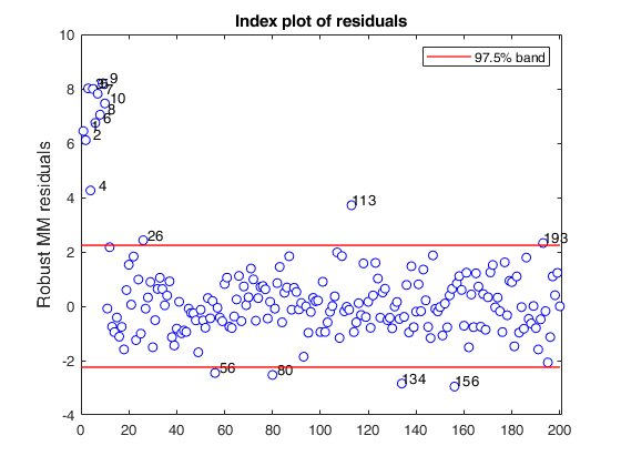
    If plots = 1, generates a plot with the robust residuals against index number. The confidence level used to draw the confidence bands for the residuals is given by the input option conflev. If conflev is not specified a nominal 0.975 confidence interval will be used.

    Example: 'plots',0

    Data Types: single | double

    yxsave —the response vector y and data matrix X are saved into the output structure out.scalar.

    Default is 0, i.e. no saving is done.

    Example: 'yxsave',1

    Data Types: double

    Output Arguments

    expand all

    out — description Structure

    A structure containing the following fields

    Value Description
    beta

    p x 1 vector. Estimate of beta coefficients after refsteps refining steps

    residuals

    n x 1 vector containing the estimates of the robust scaled residuals

    outliers

    A vector containing the list of the units declared as outliers using confidence level specified in input scalar conflev

    conflev

    Confidence level that was used to declare outliers

    weights

    n x 1 vector. Weights assigned to each observation

    rhofunc

    string identifying the rho function which has been used.

    rhofuncparam

    vector which contains the additional parameters for the specified rho function which have been used. For hyperbolic rho function the value of k =sup CVC. For Hampel rho function the parameters a, b and c. This field is empty if rhofunc is not 'hampel' or 'hyperbolic'.

    y

    response vector y. The field is present only if option yxsave is set to 1.

    X

    data matrix X. The field is present only if option yxsave is set to 1.

    class

    'MMreg'

    More About

    expand all

    Additional Details

    It does iterative reweighted least squares (IRWLS) steps from "initial beta" (b0) keeping the estimate of the scale (auxscale) fixed.

    References

    Maronna, R.A., Martin D. and Yohai V.J. (2006), "Robust Statistics, Theory and Methods", Wiley, New York.

    Acknowledgements

    This function follows the lines of MATLAB/R code developed during the years by many authors.

    For more details see the R library robustbase http://robustbase.r-forge.r-project.org/.

    The core of these routines, e.g. the resampling approach, however, has been completely redesigned, with considerable increase of the computational performance.

    See Also

    This page has been automatically generated by our routine publishFS