ctlcurvesplot
ctlcurvesplot plots the output of routine ctlcurves
Description
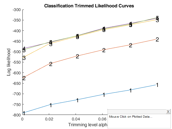
ctlcurvesplot takes as input the output of function ctlcurves (that is a series of matrices which contain the values of the CTL bands, the set of tentative solutions found using the intersection of the bands, and the likelihood ratio tests for testing k vs k+1 given alpha.
The plot enables interaction in the sense that, if option databrush has been activated, it is possible to click on a point in the plot of the ctlcurves and to see the associated classification in the scatter plot matrix.
ctlcurves and Portofino plot for the Gyeser data with all default options.outCTLnew
=ctlcurvesplot(outCTL)
Interactive_example
Example of the use of option databrush.outCTLnew
=ctlcurvesplot(outCTL,
Name, Value)
Examples
 ctlcurves and Portofino plot for the Gyeser data with all default options.
ctlcurves and Portofino plot for the Gyeser data with all default options.
Y=load('geyser2.txt');
outCTl=ctlcurves(Y,'plots',false,'nsamp',20)
ctlcurvesplot(outCTl);
k=1
k=2
k=3
k=4
k=5
Bands k=1
Bands k=2
Bands k=3
Bands k=4
Bands k=5
outCTl =
struct with fields:
Mu: {5×6 cell}
Sigma: {5×6 cell}
Pi: {5×6 cell}
IDX: {5×6 cell}
CTL: [5×6 double]
CTLbands: [5×6×60 double]
CTLlikLB: [5×6 double]
CTLlik050: [5×6 double]
CTLlikUB: [5×6 double]
CTLoptimalIDX: [271×1 double]
CTLoptimalAlpha: 0.0200
CTLoptimalK: 3
CTLtentSol: [2×4 double]
LRTpval: [4×6 table]
LRTtentSol: [2×8 double]
LRTtentSolt: [2×8 table]
LRTtentSolIDX: [271×2 double]
LRToptimalK: [2×1 double]
LRToptimalAlpha: [2×1 double]
LRToptimalIDX: [271×2 double]
kk: [1 2 3 4 5]
alpha: [0 0.0200 0.0400 0.0600 0.0800 0.1000]
Y: [271×2 double]
tclustPAR: [1×1 struct]

Interactive example 1.
Example of the use of option databrush.
%   (brushing is done only once using a rectangular selection tool)
%  Use the geyser data.
Y=load('geyser2.txt');
databrush=struct;
databrush.selectionmode='Rect';
outCTl=ctlcurves(Y,'plots',false,'nsamp',20)
ctlcurvesplot(outCTl,'databrush',databrush);
Related Examples
Interactive example 2.
Example of the use of option databrush.
%   (brushing is persistent)
%  Use the geyser data.
Y=load('geyser2.txt');
databrush=struct;
databrush.persist='on';
outCTl=ctlcurves(Y,'plots',false,'nsamp',20)
ctlcurvesplot(outCTl,'databrush',databrush);
Input Arguments
outCTL — output structure produced by function ctlcurves.
Structure.
It contains the following fields.
| Value | Description |
|---|---|
Mu |
cell of size length(kk)-by-length(alpha) containing the estimate of the centroids for each value of k and each value of alpha. More precisely, suppose kk=1:4 and alpha=[0 0.05 0.1], out.Mu{2,3} is a matrix with two rows and v columns containing the estimates of the centroids obtained when alpha=0.1. |
Sigma |
cell of size length(kk)-by-length(alpha) containing the estimate of the covariance matrices for each value of k and each value of alpha. More precisely, suppose kk=1:4 and alpha=[0 0.05 0.1], out.Sigma{2,3} is a 3D array of size v-by-v-by-2 containing the estimates of the covariance matrices obtained when alpha=0.1. |
Pi |
cell of size length(kk)-by-length(alpha) containing the estimate of the group proportions for each value of k and each value of alpha. More precisely, suppose kk=1:4 and alpha=[0 0.05 0.1], out.Pi{2,3} is a 3D array of size v-by-v-by-2 containing the estimates of the covariance matrices obtained when alpha=0.1. |
IDX |
cell of size length(kk)-by-length(alpha) containing the final assignment for each value of k and each value of alpha. More precisely, suppose kk=1:4 and alpha=[0 0.05 0.1], out.IDX{2,3} is a vector of length(n) containing the containinig the assignment of each unit obtained when alpha=0.1. Elements equal to zero denote unassigned units. |
CTL |
matrix of size length(kk)-by-length(alpha) containing the values of the trimmed likelihood curves for each value of k and each value of alpha. This output (and all the other output below which start with CTL) are present only if input option bands is true or is a struct. All the other fields belo |
CTLbands |
3D array of size length(kk)-by-length(alpha)-by-nsimul containing the nsimul replicates of out.CTL. |
CTLlikLB |
matrix of size length(kk)-by-length(alpha) containing the lower confidence bands of the trimmed likelihood curves for each value of k and each value of alpha. |
CTLlikUB |
matrix of size length(kk)-by-length(alpha) containing the upper confidence bands of the trimmed likelihood curves for each value of k and each value of alpha. T |
CTLlik050 |
matrix of size length(kk)-by-length(alpha) containing the central confidence bands of the trimmed likelihood curves for each value of k and each value of alpha. |
CTLtentSol |
matrix with size m-by-4. Details of the ordered solutions where there was intersection between two consecutive trimmed likelihood curves. First column contains the value of k, second column the value of alpha, third column the index associated to the best value of alpha, fourth colum index associated with the best value of kk. |
CTLoptimalAlpha |
scalar, optimal value of trimming. |
CTLoptimalK |
scalar, optimal number of clusters, stored as a positive integer value. |
CTLoptimalIDX |
n-by-1 vector containing assignment of each unit to each of the k groups in correspodence of OptimalAlpha and OptimalK. Cluster names are integer numbers from 1 to k. 0 indicates trimmed observations. The fields which follow which start with LRT refer to the likilhood ratio test |
LRTpval |
table with size length(kk)-1-times-length(alpha) which stores the relative frequency in which the Likelihood ratio test is greater than the corresponding bootstrap test. as a positive integer value. |
LRTtentSol |
matrix with size m-by-8. Details of the ordered solutions using the likelihood ratio test. First column (index): the index number of the solution. Second column (k): the value of k. Third column (alpha): the value of alpha. Fourth column (Truesol) contains 1 if the p-value beyond the threshold is always above $k$ shown in the second column for all $k^* >k$ else it contains 0. Fifth and sixth columns (kindex and alphaindex) contain the index numbers of optimal input values kk and alpha. Seventh column (kbestGivenalpha) contains 1 in correspondence of the best solution for each value of k (given alpha). Eight column (ProperSize) contains 1 if the solution which has been found has a minimum group size which is greater than n*max(alpha). |
LRTtentSolt |
table with the same size of LRTtentSol containing the same information of array out.TentSolLR in table format. |
LRTtentSolIDX |
matrix with size n-by-size(out.LRTtentSol,1) with the allocation associated with the tentative solutions found in out.LRTtentSol. First column refers to solution in row 1 of out.LRTtentSol ... |
LRToptimalAlpha |
scalar, optimal value of trimming. |
LRToptimalK |
scalar, optimal number of clusters, stored as a positive integer value. |
LRToptimalIDX |
n-by-r vector containing assignment of each unit to each of the k groups in correspondence of OptimalAlpha and OptimalK. Cluster names are integer numbers from 1 to k. 0 indicates trimmed observations. The fields which follow which start with LRT refer to the likelihood ratio test. |
kk |
vector containing the values of k (number of components) which have been considered. This vector is equal to input optional argument kk if kk had been specified else it is equal to 1:5. |
alpha |
vector containing the values of the trimming level which have been considered. This vector is equal to input optional argument alpha. |
tclustPAR |
a structure containing all the parameters used by tclust (restrfactor, mixt, restrtype. refsteps, equalweights, reftol, cshape, nsamp, nsampExtra, outliersFromUniform, nsimulExtra and usepriorSolExtra). |
Y |
Original data matrix Y. The field is present if option |
Data Types: struct
Name-Value Pair Arguments
Specify optional comma-separated pairs of Name,Value arguments.
Name is the argument name and Value
is the corresponding value. Name must appear
inside single quotes (' ').
You can specify several name and value pair arguments in any order as
Name1,Value1,...,NameN,ValueN.
 'crit',0.05
, 'thresh',0.10
, 'tag','myplot'
, 'tag','myplot1'
, 'conflev',0.9
, 'datatooltip',''
, 'databrush',1
, 'nameY',{'myY1', 'myY2'}
crit
—criterion for sgnificance.scalar in the in interval (0 1) | empty value.
Scalar which defines the p-value threshold to define a solution as significant and to reject the null hypothesis of smaller groups in the likelihood ratio test. For example when crit is 0.05 when we test $k$ against $k+1$ given a certain value of $\alpha$, if the empirical p-value is greater than crit we accept the null hypothesis of $k$ groups. The default value of crit is empty, that is we do not change the tentative solutions found by producere ctlcurves.
Example: 'crit',0.05
Data Types: double
thresh
—threshold which defines where to put NaN in the
out.pvalLRtest matrix.
Scalar in the interval [0 1].
The default value is 0.05. In other words the subsequent values in a particular column of out.pvalLRtest which follow a number breater than 0.05 will be set to NaN.
Example: 'thresh',0.10
Data Types: char
tagCtl
—Personalized tag for CTL curves plot.string.
String which identifies the handle of the plot which is about to be created. The default is to use tag 'pl_Ctl' for the classification likelihood curves plot with bands.
Note that if the program finds a plot which has a tag equal to the one specified by the user, then the output of the new plot overwrites the existing one in the same window else a new window is created.
Example: 'tag','myplot'
Data Types: char
tagPortofino
—Personalized tag for Portofino plot.string.
String which identifies the handle of the plot which is about to be created. The default is to use tag 'pl_Portofino' for the Portofino plot.
Note that if the program finds a plot which has a tag equal to the one specified by the user, then the output of the new plot overwrites the existing one in the same window else a new window is created.
Example: 'tag','myplot1'
Data Types: char
conflev
—confidence level of the bands.empty value (default) | scalar.
Scalar in the interval (0 1) which contains the confidence level of the bands.
The default is to use the confidence level taken from ctlcurves (that is 50 per cent confidence level).
Example: 'conflev',0.9
Data Types: double
datatooltip
—interactive clicking.empty value (default) | structure.
The default is datatooltip=''.
If datatooltip = 1, the user can select with the mouse a solution in order to have the following information: 1) value of k which has been selected 2) value of alpha which has been selected 3) frequency distribution of the associated classification If datatooltip is a structure it may contain the following the fields
| Value | Description |
|---|---|
DisplayStyle |
Determines how the data cursor displays. datatip | window. - datatip displays data cursor information in a small yellow text box attached to a black square marker at a data point you interactively select. - window displays data cursor information for the data point you interactively select in a floating window within the figure. |
SnapToDataVertex |
Specifies whether the data cursor snaps to the nearest data value or is located at the actual pointer position. on | off. - on data cursor snaps to the nearest data value - off data cursor is located at the actual pointer position. (see the MATLAB function datacursormode or the examples below). Default values are datatooltip.DisplayStyle = 'Window' and datatooltip.SnapToDataVertex = 'on'. |
Example: 'datatooltip',''
Data Types: scalar double or struct
databrush
—interactive mouse brushing.empty value, scalar | structure.
If databrush is an empty value (default), no brushing is done. The activation of this option (databrush is a scalar or a structure) enables the user to select a set of values of ctl curves in the current plot and to see the corresponding classification highlighted in the scatter plot matrix (spm). If spm does not exist it is automatically created. Please, note that the window style of the other figures is set equal to that which contains the ctl plot. In other words, if the ctl plot is docked all the other figures will be docked too.
DATABRUSH IS A SCALAR. If databrush is a scalar the default selection tool is a rectangular brush and it is possible to brush only once (that is persist='').
DATABRUSH IS A STRUCTURE. If databrush is a structure, it is possible to use all optional arguments of function selectdataFS and the following optional arguments: - databrush.persist = repeated brushing enabled. Persist is an empty value or a scalar containing the strings 'on' or 'off'.
The default value of persist is '', that is brushing is allowed only once.
If persist is 'on' or 'off' brushing can be done as many time as the user requires.
If persist='on' then the corresponding spmplot of the solutions currently brushed are added to those previously brushed.
If persist='off' every time a new brush is performed scatter plot matrices corresponding to previously brushed solutions are removed.
- dispopt = string which controls how to fill the diagonals in the scatterplot matrix of the brushed solutions. Set dispopt to 'hist' (default) to plot histograms, or 'box' to plot boxplots.
Example: 'databrush',1
Data Types: single | double | struct
nameY
—variable labels.cell array.
Cell array of strings containing the labels of the variables. As default value, the labels which are added are Y1, ..., Yv.
Example: 'nameY',{'myY1', 'myY2'}
Data Types: cell
Output Arguments
outCTLnew — description
Structure
Structure. This structure is exactly equal to input structure outCTL unless optional input option crit is specfied. In this case using the new value of crit starting from the input table of p-values outCTL.LRTpval we can obtain a new set of tentative solutions (outCTLnew.LRTtentSol outCTLnew.LRTtentSolt) and associated classification (outCTLnew.LRTtentSolIDX), a new optimal value of k (outCTLnew.LRToptimalK) a new optimal alpha (outCTLnew.LRToptimalAlpha) a new optional classification (outCTLnew.LRToptimalIDX). In what follows we shows show just the fields which might change
| Value | Description |
|---|---|
LRTtentSol |
matrix with size m-by-8. Details of the ordered solutions using the likelihood ratio test. First column (index): the index number of the solution. Second column (k): the value of k. Third column (alpha): the value of alpha. Fourth column (Truesol) contains 1 if the p-value beyond the threshold is always above $k$ shown in the second column for all $k^* >k$ else it contains 0. Fifth and sixth columns (kindex and alphaindex) contain the index numbers of optimal input values kk and alpha. Seventh column (kbestGivenalpha) contains 1 in correspondence of the best solution for each value of k (given alpha). Eight column (ProperSize) contains 1 if the solution which has been found has a minimum group size which is greater than n*max(alpha). |
LRTtentSolt |
table with the same size of LRTtentSol containing the same information of array out.TentSolLR in table format. |
LRTtentSolIDX |
matrix with size n-by-size(out.LRTtentSol,1) with the allocation associated with the tentative solutions found in out.LRTtentSol. First column refers to solution in row 1 of outCTLnew.LRTtentSol ... |
LRToptimalAlpha |
scalar, optimal value of trimming. |
LRToptimalK |
scalar, optimal number of clusters, stored as a positive integer value. |
LRToptimalIDX |
n-by-r vector containing assignment of each unit to each of the k groups in correspondence of OptimalAlpha and OptimalK. Cluster names are integer numbers from 1 to k. 0 indicates trimmed observations. The fields which follow which start with LRT refer to the likelihood ratio test. |