
|
existFS |
fanBICpn |
 |
fanBIC
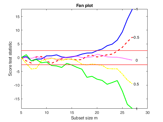
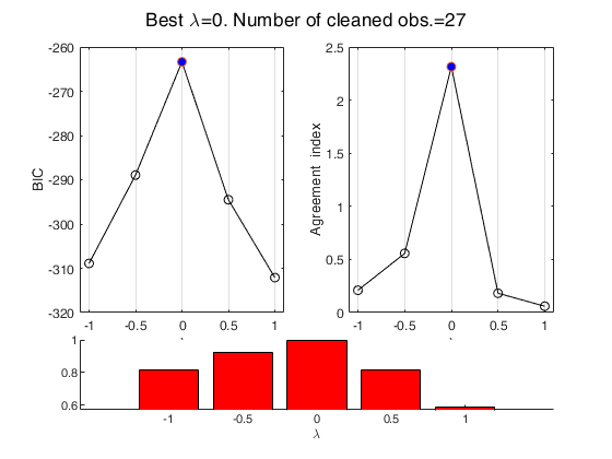
fanBIC uses the output of FSRfan to choose the best value of the transformation parameter in linear regression
Description
Examples
 fanBIC with all default options.
fanBIC with all default options.load the wool data.
XX=load('wool.txt');
y=XX(:,end);
X=XX(:,1:end-1);
% FSRfan and fanplotFS with all default options
[outFSR]=FSRfan(y,X,'msg',0);
out=fanBIC(outFSR);
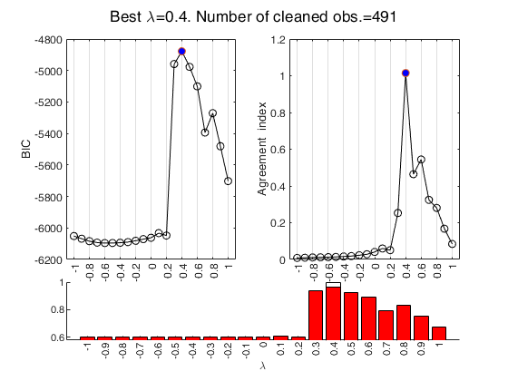
BIC plot with optional arguments.
BIC plot with optional arguments.FSRfan and fanBIC with specified lambda.
load('loyalty.txt');
y=loyalty(:,4);
X=loyalty(:,1:3);
% la = vector containing the grid of values to use for the
% transformation parameter
la=-1:0.1:1;
[outFSRfan]=FSRfan(y,X,'la',la,'msg',0,'plots',0);
out=fanBIC(outFSRfan);
Input Arguments
Output Arguments
References
Atkinson, A.C. and Riani, M. (2000), "Robust Diagnostic Regression Analysis", Springer Verlag, New York.
Atkinson, A.C. and Riani, M. (2002a), Tests in the fan plot for robust, diagnostic transformations in regression, "Chemometrics and Intelligent Laboratory Systems", Vol. 60, pp. 87-100.
Atkinson, A.C. Riani, M., Corbellini A. (2019), The analysis of transformations for profit-and-loss data, Journal of the Royal Statistical Society, Series C, "Applied Statistics", https://doi.org/10.1111/rssc.12389
Atkinson, A.C. Riani, M. and Corbellini A. (2021), The Box–Cox Transformation: Review and Extensions, "Statistical Science", Vol. 36, pp. 239-255, https://doi.org/10.1214/20-STS778