mdpdR
mdpdR allows to apply Minimum Density Power Divergence criterion to parametric regression problems.
Description
Examples
Call of mdpdR with all default options.
Simulate a regression model.
rng('default')
rng(1000)
n=1000;
p=3;
sig=0.01;
eps=randn(n,1);
X=randn(n,p);
bet=3*ones(p,1);
y=X*bet+sig*eps;
[out] = mdpdR(y, X, 0.01);
Example of use of option yxsave.
Simulate a regression model.
n=100;
p=3;
sig=0.01;
eps=randn(n,1);
X=randn(n,p);
bet=3*ones(p,1);
y=X*bet+sig*eps;
% Contaminate the first 10 observations.
y(1:10)=y(1:10)+0.05;
[out] = mdpdR(y, X, 1,'yxsave',1);
resindexplot(out)
Related Examples
 Compare MLE estimator with MDPD estimator (uncontaminated data).
Compare MLE estimator with MDPD estimator (uncontaminated data).Scenario, as in example 1, of Durio and Isaia (2011).
% 600 points generated according to the model
% Y=0.5*X1+0.5*X2+eps
% and n2 = 120 points (outliers), drawn from the model
% X1,X2~U(0,1) eps~N(0,0.1^2)
close all;
n   = 600;
p   = 2;
sig = 0.1;
eps = randn(n,1);
X   = rand(n,p);
bet = 0.5*ones(p,1);
y   = X*bet+sig*eps;
[outalpha1] = mdpdR(y, X, 1);
h1 = subplot(2,1,1);
resindexplot(outalpha1,'h',h1);
title('alpha=1','FontSize',15);
h2 = subplot(2,1,2);
[outalpha0] = mdpdR(y, X, 0);
resindexplot(outalpha0,'h',h2);
title('alpha=0','FontSize',15);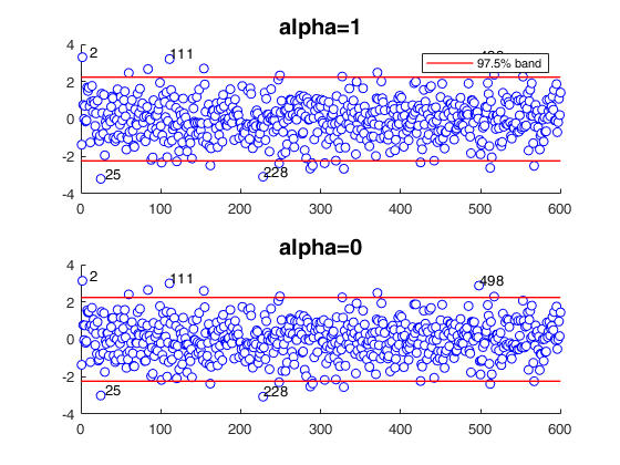
Compare MLE estimator with MDPD estimator (EX2).
Scenario, as in example 2, of Durio and Isaia (2011).
% 480 points generated according to the model
% Y=0.5*X1+0.5*X2+eps
% and n2 = 120 points (outliers), drawn from the model
% Y =0.7X1 +0.7X2 + eps
% X1,X2~U(0,1) eps~N(0,0.1^2)
close all;
sig  = 0.1;
p    = 2;
n1   = 480;
eps1 = randn(n1,1);
X1   = rand(n1,p);
bet1 = 0.5*ones(p,1);
y1   = X1*bet1+sig*eps1;
n2   = 120;
eps2 = randn(n2,1);
X2   = rand(n2,p);
bet2 = 0.7*ones(p,1);
y2   = X2*bet2+sig*eps2;
y    = [y1;y2];
X    = [X1;X2];
n=n1+n2;
group=2*ones(n,1);
group(1:n1)=1;
yXplot(y,X,group)
[out] = mdpdR(y, X, 1);
h1 = subplot(2,1,1);
resindexplot(out,'h',h1);
title('alpha=1','FontSize',15);
h2 = subplot(2,1,2);
[outalpha0] = mdpdR(y, X, 0);
resindexplot(outalpha0,'h',h2);
title('alpha=0','FontSize',15)
varnames={'MLE alpha=0' 'MD alpha=1'};
if verLessThan('matlab', '9.7.0')
varnames=matlab.lang.makeValidName(varnames);
end
% Compare robust and MLE estimate
disp(table(outalpha0.beta,out.beta,'VariableNames',varnames))
Compare MLE estimator with MDPD estimator (EX3).
Scenario, as in example 3, of Durio and Isaia (2011).
% 480 points generated according to the model
% Y=0.25*X1+0.25*X2+0.25*X3+0.25*X4+eps
% and n2 = 120 points (outliers), drawn from the model
% Y=0.35*X1+0.35*X2+0.35*X3+0.35*X4+eps
% X1,X2,X3,X4~U(0,1) eps~N(0,0.1^2)
close all;
sig  = 0.1;
p    = 4;
n1   = 480;
eps1 = randn(n1,1);
X1   = rand(n1,p);
bet1 = 0.25*ones(p,1);
y1   = X1*bet1+sig*eps1;
n2   = 120;
eps2 = randn(n2,1);
X2   = rand(n2,p);
bet2 = 0.35*ones(p,1);
y2   = X2*bet2+sig*eps2;
y    = [y1;y2];
X    = [X1;X2];
n = n1+n2;
group= 2*ones(n,1);
group(1:n1)=1;
yXplot(y,X,group)
[out] = mdpdR(y, X, 1);
h1 = subplot(2,1,1);
resindexplot(out,'h',h1);
title('alpha=1','FontSize',15);
h2=subplot(2,1,2);
% MLE estimate
[outalpha0] = mdpdR(y, X, 0);
resindexplot(outalpha0,'h',h2);
title('alpha=0','FontSize',15);
% Compare robust and MLE estimate
varnames={'MLE alpha=0' 'MD alpha=1'};
if verLessThan('matlab', '9.7.0')
varnames=matlab.lang.makeValidName(varnames);
end
disp(table(outalpha0.beta,out.beta,'VariableNames',varnames))
Compare MLE estimator with MDPD estimator (EX4).
% Compare MLE estimator with MDPD estimator (EX4).
% Scenario, as in example 4, of Durio and Isaia (2011).
% 180 points generated according to the model
% Y  = 0.25*X1+eps
% X1~U(0,0.5) eps~N(0,0.1^2)
% and n2 = 20 points (outliers), drawn from the model
% Y  = 0.25*X2+eps
% X2~U(0.5,1) eps~N(0,0.1^2)
% and m points (m=5, 10, 20, 30 40, 50)
% Y  = 0.7*X3+eps3
% X3~U(0.7,1) eps3~N(0,0.05^2)
close all;
sig  = 0.1;
p    = 1;
n1   = 180;
eps1 = randn(n1,1);
X1   = rand(n1,p)*0.5;
y1   = X1+sig*eps1;
n2   = 20;
eps2 = randn(n2,1);
X2   = rand(n2,p)*0.5+0.5;
y2   = X2+sig*eps2;
% Additional m points
m    = 5;
X3   = rand(m,p)*0.3+0.7;
eps3 = randn(m,1);
y3   = X3+0.05*eps3;
y    = [y1;y2;y3];
X    = [X1;X2;X3];
group= 3*ones(n1+n2+m,1);
group(1:n1)=1;
group(n1+1:n1+n2)=2;
yXplot(y,X,group)
[out] = mdpdR(y, X, 1);
h1=subplot(2,1,1);
resindexplot(out,'h',h1);
title('alpha=1','FontSize',15);
n=n1+n2;
h2=subplot(2,1,2);
% MLE estimate
[outalpha0] = mdpdR(y, X, 0);
resindexplot(outalpha0,'h',h2);
title('alpha=0','FontSize',15);
% Compare robust and MLE estimate
varnames={'MLE alpha=0' 'MD alpha=1'};
if verLessThan('matlab', '9.7.0')
varnames=matlab.lang.makeValidName(varnames);
end
disp(table(outalpha0.beta,out.beta,'VariableNames',varnames))
MPDP applied to Forbes data.
MPDP applied to Forbes data.Interactive_example
clearvars;close all;
% scatterplot of data: one point looks outlying
load('forbes.txt');
y=forbes(:,2);
X=forbes(:,1);
h1=subplot(2,1,1);
[out] = mdpdR(y, X, 1);
resindexplot(out,'h',h1);
title('alpha=1','FontSize',15);
h2=subplot(2,1,2);
% MLE estimate
[outalpha0] = mdpdR(y, X, 0);
resindexplot(outalpha0,'h',h2);
title('alpha=0','FontSize',15);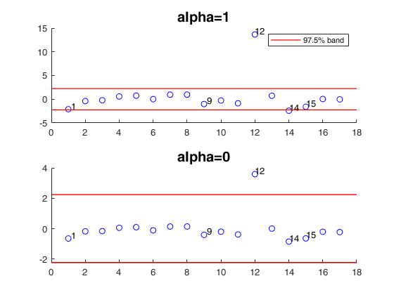
mdpdR applied to the Belgium telephone data.
This dataset concerns the number of international calls from Belgium, taken from the Belgian Statistical Survey, published by the Ministry of Economy. This dataset consists in 24 observations on the following 2 variables.
% Year (1950 - 1973)
% Calls (Number of Calls in tens of millions)
% Source Rousseeuw P.J. and  Leroy A.M. (1987), Robust Regression and
% Outlier Detection; Wiley, page 26, table 2.
XX=[50  0.44
51  0.47
52  0.47
53  0.59
54  0.66
55  0.73
56  0.81
57  0.88
58  1.06
59  1.20
60  1.35
61  1.49
62  1.61
63  2.12
64 11.90
65 12.40
66 14.20
67 15.90
68 18.20
69 21.20
70  4.30
71  2.40
72  2.70
73  2.90];
y=XX(:,2);
X=XX(:,1);
out=mdpdR(y,X,0);
Input Arguments
y — Response variable.
Vector.
Response variable, specified as a vector of length n, where n is the number of observations. Each entry in y is the response for the corresponding row of X.
Missing values (NaN's) and infinite values (Inf's) are allowed, since observations (rows) with missing or infinite values will automatically be excluded from the computations.
Data Types: double
X — Predictor variables.
Matrix.
Matrix of explanatory variables (also called 'regressors') of dimension n x (p-1) where p denotes the number of explanatory variables including the intercept.
Rows of X represent observations, and columns represent variables. By default, there is a constant term in the model, unless you explicitly remove it using input option intercept, so do not include a column of 1s in X. Missing values (NaN's) and infinite values (Inf's) are allowed, since observations (rows) with missing or infinite values will automatically be excluded from the computations.
Data Types: double
alpha — tuning parameter.
Non negative scalar in the interval (0 1].
The robustness of the Minimum Density Power Divergence estimator increases as the tuning parameter $\alpha$ increases, but at the same time its efficiency decreases (Basu et al., 1998). For $\alpha=0$ the MDPDE becomes the Maximum Likelihood estimator, while for $\alpha=1$ the divergence yields the $L_2$ metric and the estimator minimizes the $L_2$ distance between the densities, e.g., Scott (2001), Durio and Isaia (2003).
Data Types: double
Name-Value Pair Arguments
Specify optional comma-separated pairs of Name,Value arguments.
Name is the argument name and Value
is the corresponding value. Name must appear
inside single quotes (' ').
You can specify several name and value pair arguments in any order as
Name1,Value1,...,NameN,ValueN.
 'beta0',[0.5 0.2 0.1]
, 'intercept',true
, 'dispresults',false
, 'conflev',0.99
, 'plots',0
, 'yxsave',1
, 'MaxIter',100
, 'TolX',1e-8
modelfun
—non linear function to use.it is a function_handle | an empty value (default).
If modelfun is empty, the link between $X$ and $\beta$ is assumed to be linear, otherwise it is necessary to specify a function (using @) that accepts two arguments, a coefficient vector and the array X and returns the vector of fitted values from the non linear model y. For example, to specify the hougen (Hougen-Watson) nonlinear regression function, use the function handle @hougen.
Example: 'modelfun', modelfun
where modelfun = @(beta,X) X*beta(1).*exp(-beta(2)*X);
Data Types: function_handle or empty value.
theta0
—Initial point.vector | empty value.
Empty value or vector containing initial values for the coefficients (beta0 and sigma0) just in case modelfun is non empty. If modelfun is empty this argument is ignored.
Example: 'beta0',[0.5 0.2 0.1]
Data Types: double
intercept
—Indicator for constant term.true (default) | false.
If true, and modelfun is empty (that is, if the link between X and beta is linear) a model with constant term will be fitted (default), else no constant term will be included.
This argument is ignored if modelfun is not empty.
Example: 'intercept',true
Data Types: boolean
dispresults
—Display results on the screen.boolean.
If dispresults is true (default), it is possible to see on the screen table Btable.
Example: 'dispresults',false
Data Types: Boolean
conflev
—Confidence level which is used to declare units as outliers.scalar.
Usually conflev=0.95, 0.975 0.99 (individual alpha) or 1-0.05/n, 1-0.025/n, 1-0.01/n (simultaneous alpha). Default value is 0.975
Example: 'conflev',0.99
Data Types: double
plots
—Plot on the screen.scalar.
If plots = 1, generates a plot with the residuals against index number. The confidence level used to draw the confidence bands for the residuals is given by the input option conflev. If conflev is not specified a nominal 0.975 confidence interval is used.
Example: 'plots',0
Data Types: single | double
yxsave
—store X and y.scalar.
Scalar that is set to 1 to request that the response vector y and data matrix X are saved into the output structure out. Default is 0, i.e. no saving is done.
Example: 'yxsave',1
Data Types: double
MaxIter
—maximum number of iterations allowed.positive integer.
The default value is 1000
Example: 'MaxIter',100
Data Types: double
TolX
—Tolerance for declaring convergence.scalar.
The default value of TolX is 1e-7.
Example: 'TolX',1e-8
Data Types: double
Output Arguments
out — description
Structure
A structure containing the following fields
| Value | Description |
|---|---|
beta |
vector containing the MPDP estimator of regression coefficients. |
scale |
scalar containing the estimate of the scale (sigma). |
residuals |
n x 1 vector containing the estimates of the scaled residuals. The residuals are robust or not depending on the input value alpha. |
fittedvalues |
n x 1 vector containing the fitted values. |
outliers |
this output is present only if conflev has been specified. It is a vector containing the list of the units declared as outliers using confidence level specified in input scalar conflev. |
conflev |
confidence level which is used to declare outliers. Remark: scalar out.conflev will be used to draw the horizontal line (confidence band) in the plot. |
y |
response vector Y. The field is present only if option yxsave is set to 1. |
X |
data matrix X. The field is present only if option yxsave is set to 1. |
class |
'Sreg' |
Btable |
table containing estimated beta coefficients, standard errors, t-stat and p-values. The content of matrix B is as follows: 1st col = beta coefficients and sigma (in the last element). This output is present only if input option dispresults is true. 2nd col = standard errors; 3rd col = t-statistics; 4th col = p-values. |
exitflag |
Reason fminunc or fminsearch stopped. Integer. A value greater then 0 denotes normal convergence. See help of functions fminunc or fminsearch for further details. |
More About
Additional Details
We assume that the random variables $Y|x$ are distributed as normal $N( \eta(x,\beta), \sigma_0)$ random variable with density function $\phi$.
Note that, if the model is linear $\eta(x,\beta)= x^T \beta$. The estimate of the vector $\theta_\alpha=(\beta_1, \ldots, \beta_p)^T$ (Minimum Density Power Divergence Estimate) is given by:
\[ \mbox{argmin}_{\beta, \sigma} \left[ \frac{1}{\sigma^\alpha \sqrt{ (2 \pi)^\alpha(1+\alpha)}}-\frac{\alpha+1}{\alpha} \frac{1}{n} \sum_{i=1}^n \phi^\alpha (y_i| \eta (x_i, \beta), \sigma) \right] \] As the tuning parameter $\alpha$ increases, the robustness of the Minimum Density Power Divergence Estimator (MDPDE) increases, while its efficiency decreases (Basu et al. 1998). For $\alpha=0$ the MDPDE becomes the Maximum Likelihood Estimator, while for $\alpha=1$ the estimator minimizes the $L_2$ distance between the densities (Durio and Isaia, 2003),References
Basu, A., Harris, I.R., Hjort, N.L. and Jones, M.C., (1998), Robust and efficient estimation by minimizing a density power divergence, "Biometrika", Vol. 85, pp. 549-559.
69-83.
Durio A., Isaia E.D. (2011), The Minimum Density Power Divergence Approach in Building Robust Regression Models, "Informatica", Vol. 22, pp. 43-56.