mdpdReda

mdpdReda allows to monitor Minimum Density Power Divergence criterion to parametric regression problems.

Syntax

Description

example

out =mdpdReda(y, X) Call of mdpdReda with all default options.

example

out =mdpdReda(y, X, Name, Value) Example of use of option alpha.

Examples

expand all

  • Call of mdpdReda with all default options.
  • Simulate a regression model.

    n=100;
    p=3;
    sig=0.01;
    eps=randn(n,1);
    X=randn(n,p);
    bet=3*ones(p,1);
    y=X*bet+sig*eps;
    % Contaminate the first 10 observations.
    y(1:10)=y(1:10)+0.05;
    [out] = mdpdReda(y, X,'plots',1);

  • Example of use of option alpha.
  • n=100;
    p=3;
    sig=0.01;
    eps=randn(n,1);
    X=randn(n,p);
    bet=3*ones(p,1);
    y=X*bet+sig*eps;
    % Contaminate the first 10 observations.
    y(1:10)=y(1:10)+0.05;
    [out] = mdpdReda(y, X,'plots',1,'alphaORbdp','alpha','tuningpar',[1 0.8 0.2 0]);

    Related Examples

    expand all

  • mdpdReda applied to example 1 of Durio and Isaia (2011).
  • 600 points generated according to the model Y=0.5*X1+0.5*X2+eps and n2 = 120 points (outliers), drawn from the model X1,X2~U(0,1) eps~N(0,0.1^2)

    n=600;
    p=2;
    sig=0.1;
    eps=randn(n,1);
    X=rand(n,p);
    bet=0.5*ones(p,1);
    y=X*bet+sig*eps;
    [out] = mdpdReda(y,X ,'plots',1);

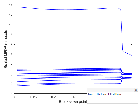
  • mdpdReda applied to Forbes data.
  • load('forbes.txt');
    y=forbes(:,2);
    X=forbes(:,1);
    [outalpha0] = mdpdReda(y, X, 'plots',1);
    Click here for the graphical output of this example (link to Ro.S.A. website)

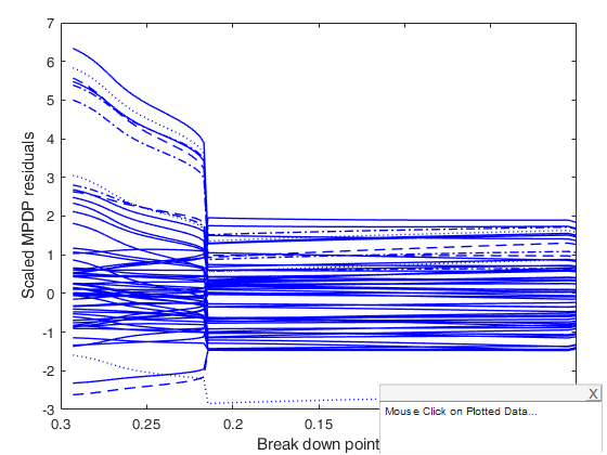
  • mdpdReda applied to multiple regression data.
  • load('multiple_regression.txt');
    y=multiple_regression(:,4);
    X=multiple_regression(:,1:3);
    [out] = mdpdReda(y, X, 'plots',1);
    Click here for the graphical output of this example (link to Ro.S.A. website)

    Input Arguments

    expand all

    y — Response variable. Vector.

    Response variable, specified as a vector of length n, where n is the number of observations. Each entry in y is the response for the corresponding row of X.

    Missing values (NaN's) and infinite values (Inf's) are allowed, since observations (rows) with missing or infinite values will automatically be excluded from the computations.

    Data Types: double

    X — Predictor variables. Matrix.

    Matrix of explanatory variables (also called 'regressors') of dimension n x (p-1) where p denotes the number of explanatory variables including the intercept.

    Rows of X represent observations, and columns represent variables. By default, there is a constant term in the model, unless you explicitly remove it using input option intercept, so do not include a column of 1s in X. Missing values (NaN's) and infinite values (Inf's) are allowed, since observations (rows) with missing or infinite values will automatically be excluded from the computations.

    Data Types: double

    Name-Value Pair Arguments

    Specify optional comma-separated pairs of Name,Value arguments. Name is the argument name and Value is the corresponding value. Name must appear inside single quotes (' '). You can specify several name and value pair arguments in any order as Name1,Value1,...,NameN,ValueN.

    Example: 'tuningpar',[1 0.8 0.5 0.4 0.3 0.2 0.1] , 'alphaORbdp','bdp' , 'modelfun', modelfun where modelfun = @(beta,X) X*beta(1).*exp(-beta(2)*X); , 'beta0',[0.5 0.2 0.1] , 'intercept',true , 'conflev',0.99 , 'plots',0

    tuningpar —tuning parameter.scalar | Vector.

    tuningpar may refer to $\alpha$ (default) or to breakdown point (depending on input option alphaORbdp.

    As the tuning parameter $\alpha$ (bdp) decreases the robustness of the Minimum Density Power Divergence estimator decreases while its efficiency increases (Basu et al., 1998). For $\alpha=0$ the MDPDE becomes the Maximum Likelihood estimator, while for $\alpha=1$ the divergence yields the $L_2$ metric and the estimator minimizes the $L_2$ distance between the densities, e.g., Scott (2001), Durio and Isaia (2003). The sequence is forced to be monotonically decreasing, e.g. alpha=[1 0.9 0.5 0.01]. The default for tuningpar is a sequence from 1 to 0 with step -0.01.

    Example: 'tuningpar',[1 0.8 0.5 0.4 0.3 0.2 0.1]

    Data Types: double

    alphaORbdp —ctuning refers to $\alpha$ or to breakdown point.character.

    Character which specifies what are the values in input option tuningpar. If this option is not specified or it is equal to 'alpha' then program assumes that the values of tuningpar refer to 'alpha', elseif this option is equal to 'bdp', program assumes that the values of tuninpar refer to breakdownpoint.

    Example: 'alphaORbdp','bdp'

    Data Types: char

    modelfun —non linear function to use.function_handle | empty value (default).

    If modelfun is empty the link between $X$ and $\beta$ is assumed to be linear else it is necessary to specify a function (using @) that accepts two arguments, a coefficient vector and the array X and returns the vector of fitted values from the non linear model y. For example, to specify the hougen (Hougen-Watson) nonlinear regression function, use the function handle @hougen.

    Example: 'modelfun', modelfun where modelfun = @(beta,X) X*beta(1).*exp(-beta(2)*X);

    Data Types: function_handle or empty value

    theta0 —empty value or vector containing initial values for the coefficients (beta0 and sigma0) just in case modelfun is non empty.if modelfun is empty this argument is ignored and LMS solution will be used as initial solution for the minimization.

    Example: 'beta0',[0.5 0.2 0.1]

    Data Types: double

    intercept —Indicator for constant term.true (default) | false.

    If true, and modelfun is empty (that is if the link between X and beta is linear) a model with constant term will be fitted (default), else no constant term will be included.

    This argument is ignored if modelfun is not empty.

    Example: 'intercept',true

    Data Types: boolean

    conflev —Confidence level.scalar.

    Confidence level which is used to declare units as outliers.

    Usually conflev=0.95, 0.975 0.99 (individual alpha) or 1-0.05/n, 1-0.025/n, 1-0.01/n (simultaneous alpha).

    Default value is 0.975.

    Example: 'conflev',0.99

    Data Types: double

    plots —Plot on the screen.scalar.

    If plots = 1, generates a plot of the monitoring of residuals against alpha.

    Example: 'plots',0

    Data Types: single | double

    Output Arguments

    expand all

    out — description Structure

    A structure containing the following fields

    Value Description
    Beta

    matrix containing the mpdp estimator of regression coefficients for each value of alpha

    Scale

    vector containing the estimate of the scale (sigma) for each value of alpha.

    RES

    n x length(alpha) matrix containing the robust scaled residuals for each value of bdp

    Outliers

    Boolean matrix containing the list of the units declared as outliers for each value of alpha using confidence level specified in input scalar conflev

    conflev

    confidence level which is used to declare outliers.

    alpha

    vector which contains the values of alpha which have been used. To each value of alpha corresponds a value of bdp (see out.bdp).

    bdp

    vector which contains the values of bdp which have been used. To each value of bdp corresponds a value of alpha (see out.alpha).

    y

    response vector y. The field is present if option yxsave is set to 1.

    X

    data matrix X. The field is present if option yxsave is set to 1.

    class

    'MDPDReda'

    Fval

    Value of the objective function and reason fminunc or fminsearch stopped and v. Matrix.

    length(alpha)-by-3 matrix.

    The first column contains the values of alpha which have been considered.

    The second column contains the values of the objective function at the solution.

    The third column contins the details about convergence. A value greater then 0 denotes normal convergence. See help of functions fminunc or fminsearch for further details.

    More About

    expand all

    Additional Details

    We assume that the random variables $Y|x$ are distributed as normal $N( \eta(x,\beta), \sigma_0)$ random variable with density function $\phi$.

    Note that if the model is linear $\eta(x,\beta)= x^T \beta$. The estimate of the vector $\theta_\alpha=(\beta_1, \ldots, \beta_p)^T$ (Minimum Density Power Divergence Estimate) is given by:

    \[ \mbox{argmin}_{\beta, \sigma} \left[ \frac{1}{\sigma^\alpha \sqrt{ (2 \pi)^\alpha(1+\alpha)}}-\frac{\alpha+1}{\alpha} \frac{1}{n} \sum_{i=1}^n \phi^\alpha (y_i| \eta (x_i, \beta), \sigma) \right] \] As the tuning paramter $\alpha$ increases, the robustness of the Minimum Density Power Divergence Estimator (MDPDE) increases while its efficieny decreases (Basu et al. 1998). For $\alpha=0$ the MDPDE becomes the Maximum Likelihood Estimator, while for $\alpha=1$ the estimator minimizes the $L_2$ distance between the densities (Durio and Isaia, 2003),

    References

    Basu, A., Harris, I.R., Hjort, N.L. and Jones, M.C., (1998), Robust and efficient estimation by minimizing a density power divergence, "Biometrika", Vol. 85, pp. 549-559.

    69-83.

    Durio A., Isaia E.D. (2011), The Minimum Density Power Divergence Approach in Building Robust Regression Models, "Informatica", Vol. 22, pp. 43-56.

    See Also

    |

    This page has been automatically generated by our routine publishFS