quickselectFSw_demo
quickselectFSw_demo illustrates the functioning of quickselectFSw
Syntax
Description
Examples
 quickselectFSw without optional parameter p gives the weighted
median.
quickselectFSw without optional parameter p gives the weighted
median.
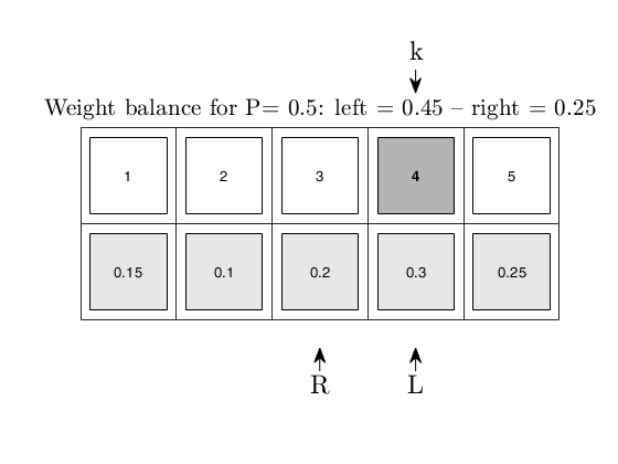
quickselectFSw without optional parameter p gives the weighted
median.The median is 3, but the weighted one is 4, corresponding to the weight 0.3.
A = [1 2 3 4 5];
W = [0.15 0.1 0.2 0.3 0.25];
i=randperm(5);
A=A(i); W=W(i);
[kD, kW , kstar] = quickselectFSw_demo(A,W);
Input Arguments
Output Arguments
References
Azzini, I., Perrotta, D. and Torti, F. (2023), A practically efficient fixed-pivot selection algorithm and its extensible MATLAB suite, "arXiv, stat.ME, eprint 2302.05705"