tBothSides

tBothSides allows users to transform both sides of a (nonlinear) regression model.

Syntax

Description

example

out =tBothSides(y, X) Call of tBothSides with all default options.

example

out =tBothSides(y, X, Name, Value) Call of tBothSides with parameter lambda fixed.

Examples

expand all

  • Call of tBothSides with all default options.
  • Load Assay data from Davidian M. and Haaland P. (1989).

    % The Relationship Between Transformation and Weighting
    % in Regression, With Application to Biological and Physical Science,
    % Institute of Statistics mimeo series Report 1947, North Carolina State University. 
    % File is downloadable from
    % https://pdfs.semanticscholar.org/7067/fd66fe06f114cac58eef8253eb7483edfd29.pdf
    % The material assayed was obtained from two sources, with every other
    % concentration starting with 0.476 from the first source and the remainder from the
    % second. Replicate observations were obtained by subsampling at each concentration.
    x=[0.476	0.924	1.905	3.696	7.619	14.874	30.474	59.134];
    yy=[0.05706	0.11781	0.25071	0.49596	1.03928	2.14635	4.24397	8.53848...
    0.057	0.11615	0.25398	0.4807	1.03659	2.09495		    8.41333...
    0.06363	0.12587	0.24552	0.49442	1.12641	2.24941	4.7011	9.01437...
    0.05566	0.12308	0.24889	0.52321	1.10456	2.19937	4.44709	8.73544...
    0.05449	0.11629	0.24858	0.49931	1.03184	2.16042	4.42707	8.33862...
    0.06153	0.11878	0.24657	0.5021	1.02598	2.09198	4.39725	8.33347...
    0.05837	0.11869	0.24212	0.4886	0.98267	2.07686	4.35511	8.35725...
    0.05388	0.11886	0.25975	0.48158	1.04321	2.06961	4.37357	8.39123...
    0.05618	0.12492	0.25311	0.4827	1.03838	2.12548	4.3204	8.3901];
    X=[x';x([1:6 8])'; repmat(x(:),7,1)];
    y=yy';
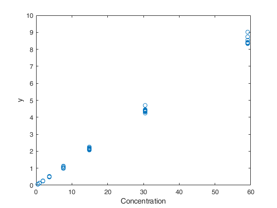
    % The plot of the data shows: a systematic increase in variance with level
    % of mean response, small variability relative to the range of the means,
    % and reasonably straight-line relationship.
    plot(X,y,'o')
    xlabel('Concentration')
    ylabel('y')
    % In this case both lambda and the beta coefficients are estimated
    % A linear link between X and beta is assumed
    out=tBothSides(y, X);
    disp(out.Btable)
                    bhat           se         tstat 
                  _________    __________    _______
    
        b1        -0.010677     0.0010009    -10.667
        b2          0.14143    0.00085986     164.47
        lambda     0.063929      0.081648    0.78298
    
    
    Click here for the graphical output of this example (link to Ro.S.A. website).

  • Call of tBothSides with parameter lambda fixed.
  • x=[0.476	0.924	1.905	3.696	7.619	14.874	30.474	59.134];
    yy=[0.05706	0.11781	0.25071	0.49596	1.03928	2.14635	4.24397	8.53848...
    0.057	0.11615	0.25398	0.4807	1.03659	2.09495		    8.41333...
    0.06363	0.12587	0.24552	0.49442	1.12641	2.24941	4.7011	9.01437...
    0.05566	0.12308	0.24889	0.52321	1.10456	2.19937	4.44709	8.73544...
    0.05449	0.11629	0.24858	0.49931	1.03184	2.16042	4.42707	8.33862...
    0.06153	0.11878	0.24657	0.5021	1.02598	2.09198	4.39725	8.33347...
    0.05837	0.11869	0.24212	0.4886	0.98267	2.07686	4.35511	8.35725...
    0.05388	0.11886	0.25975	0.48158	1.04321	2.06961	4.37357	8.39123...
    0.05618	0.12492	0.25311	0.4827	1.03838	2.12548	4.3204	8.3901];
    X=[x';x([1:6 8])'; repmat(x(:),7,1)];
    y=yy';
    % In this case only the beta coefficients are estimated
    la=0.063;
    % A linear link between X and beta is assumed
    out=tBothSides(y, X,'la',la);

    Related Examples

    expand all

  • Example of tBothSides with non linear link between X and beta.
  • Load spawners data (table 4.1 p. 141 Book CR) year spawner (S) recruiter (R) Model is R = \beta_1 S exp ( - \beta_2 S) = f_RK(S, \beta)

    XX=[1940 963 2215
    1941 572 1334
    1942 305 800
    1943 272 438
    1944 824 3071
    1945 940 957
    1946 486 934
    1947 307 971
    1948 1066 2257
    1949 480 1451
    1950 393 686
    1951 176 127
    1952 237 700
    1953 700 1381
    1954 511 1393
    1955 87 363
    1956 370 668
    1957 448 2067
    1958 819 644
    1959 799 1747
    1960 273 744
    1961 936 1087
    1962 558 1335
    1963 597 1981
    1964 848 627
    1965 619 1099
    1966 397 1532
    1967 616 2086];
    % Row 12 is removed from the analysis.
    XX(12,:)=[];
    X=XX(:,2);
    y=XX(:,3);
    % Call of tBothSides non linear link between X and beta.
    % In this case modelfun (function which specifies the link between X and beta) and
    % the vector of initial regression coefficients is specified.
    % This is the spawner recruiter model. See CR for more details.
    modelfun = @(beta,X) X*beta(1).*exp(-beta(2)*X);
    % Initial value of beta coefficients
    bini=[3; 0.0009];
    % The link between X and beta is specified inside modelfun given at the end
    % of the example
    out=tBothSides(y, X,'modelfun',modelfun,'beta0',bini,'family','BoxCox','dispresults',true);
    % Plot the original values together with estimated median regression lines
    % and 90 per cent confidence interval for fitted response.
    close all
    plot(X,y,'o')
    hold('on')
    laest=out.betaout(end);
    upConfInt= normBoxCox(out.yhattra+1.65*out.scale,1,laest,'inverse',true,'Jacobian',false);
    lowConfInt= normBoxCox(out.yhattra-1.65*out.scale,1,laest,'inverse',true,'Jacobian',false);
    [Xsor,indXsor]=sort(X);
    % Plot the estimated median recruitment
    plot(Xsor,out.yhat(indXsor),'r-')
    % Plot the estimated 95th percentile of recruitment
    plot(Xsor,upConfInt(indXsor),'r--')
    % Plot the estimated 5th percentile of recruitment
    plot(Xsor,lowConfInt(indXsor),'r--')
    ylabel('Recruiters')
    xlabel('Spawners')

  • Example where only beta coefficents are estimated and initial values for beta are provided.
  • x=[0.476	0.924	1.905	3.696	7.619	14.874	30.474	59.134];
    yy=[0.05706	0.11781	0.25071	0.49596	1.03928	2.14635	4.24397	8.53848...
    0.057	0.11615	0.25398	0.4807	1.03659	2.09495		    8.41333...
    0.06363	0.12587	0.24552	0.49442	1.12641	2.24941	4.7011	9.01437...
    0.05566	0.12308	0.24889	0.52321	1.10456	2.19937	4.44709	8.73544...
    0.05449	0.11629	0.24858	0.49931	1.03184	2.16042	4.42707	8.33862...
    0.06153	0.11878	0.24657	0.5021	1.02598	2.09198	4.39725	8.33347...
    0.05837	0.11869	0.24212	0.4886	0.98267	2.07686	4.35511	8.35725...
    0.05388	0.11886	0.25975	0.48158	1.04321	2.06961	4.37357	8.39123...
    0.05618	0.12492	0.25311	0.4827	1.03838	2.12548	4.3204	8.3901];
    X=[x';x([1:6 8])'; repmat(x(:),7,1)];
    y=yy';
    % Initial value of beta coefficients
    bini=[3; 0.0009];
    % lambda is fixed
    la=-0.2;
    % modelfun is the function which specifies the link between X and beta
    % This is the spawner recruiter model. See CR for more details.
    modelfun = @(beta,X) X*beta(1).*exp(-beta(2)*X);
    out=tBothSides(y, X,'modelfun',modelfun,'beta0',bini,'la',la);

  • Example of the use of option dispresults.
  • modelfun is the function which specifies the link between X and beta This is the spawner recruiter model. See CR for more details.

    x=[0.476	0.924	1.905	3.696	7.619	14.874	30.474	59.134];
    yy=[0.05706	0.11781	0.25071	0.49596	1.03928	2.14635	4.24397	8.53848...
    0.057	0.11615	0.25398	0.4807	1.03659	2.09495		    8.41333...
    0.06363	0.12587	0.24552	0.49442	1.12641	2.24941	4.7011	9.01437...
    0.05566	0.12308	0.24889	0.52321	1.10456	2.19937	4.44709	8.73544...
    0.05449	0.11629	0.24858	0.49931	1.03184	2.16042	4.42707	8.33862...
    0.06153	0.11878	0.24657	0.5021	1.02598	2.09198	4.39725	8.33347...
    0.05837	0.11869	0.24212	0.4886	0.98267	2.07686	4.35511	8.35725...
    0.05388	0.11886	0.25975	0.48158	1.04321	2.06961	4.37357	8.39123...
    0.05618	0.12492	0.25311	0.4827	1.03838	2.12548	4.3204	8.3901];
    X=[x';x([1:6 8])'; repmat(x(:),7,1)];
    y=yy';
    % Initial value of beta coefficients
    bini=[3; 0.0009];
    modelfun = @(beta,X) X*beta(1).*exp(-beta(2)*X);
    out=tBothSides(y, X,'modelfun',modelfun,'dispresults',true,'beta0',bini);
    % modelfun is the function which specifies the link between X and beta
    %     % This is the spawner recruiter model
    %     function [yhat]=modelfun(beta, X)
    %     yhat=X*beta(1).*exp(-beta(2)*X);
    %     end

  • Example of the use of option prolik.
  • This is the spawner recruiter model. See CR for more details.

    % modelfun is the function which specifies the link between X and beta
    x=[0.476	0.924	1.905	3.696	7.619	14.874	30.474	59.134];
    yy=[0.05706	0.11781	0.25071	0.49596	1.03928	2.14635	4.24397	8.53848...
    0.057	0.11615	0.25398	0.4807	1.03659	2.09495		    8.41333...
    0.06363	0.12587	0.24552	0.49442	1.12641	2.24941	4.7011	9.01437...
    0.05566	0.12308	0.24889	0.52321	1.10456	2.19937	4.44709	8.73544...
    0.05449	0.11629	0.24858	0.49931	1.03184	2.16042	4.42707	8.33862...
    0.06153	0.11878	0.24657	0.5021	1.02598	2.09198	4.39725	8.33347...
    0.05837	0.11869	0.24212	0.4886	0.98267	2.07686	4.35511	8.35725...
    0.05388	0.11886	0.25975	0.48158	1.04321	2.06961	4.37357	8.39123...
    0.05618	0.12492	0.25311	0.4827	1.03838	2.12548	4.3204	8.3901];
    X=[x';x([1:6 8])'; repmat(x(:),7,1)];
    y=yy';
    % Initial value of beta coefficients
    bini=[3; 0.0009];
    modelfun = @(beta,X) X*beta(1).*exp(-beta(2)*X);
    out=tBothSides(y, X,'modelfun',modelfun,'prolik',true,'beta0',bini);

    Input Arguments

    expand all

    y — Response variable. Vector.

    Response variable, specified as a vector of length n, where n is the number of observations. Each entry in y is the response for the corresponding row of X.

    Missing values (NaN's) and infinite values (Inf's) are allowed, since observations (rows) with missing or infinite values will automatically be excluded from the computations.

    Data Types: single| double

    X — Predictor variables. Matrix.

    Matrix of explanatory variables (also called 'regressors') of dimension n x (p-1) where p denotes the number of explanatory variables including the intercept.

    Rows of X represent observations, and columns represent variables. By default, there is a constant term in the model, unless you explicitly remove it using input option intercept, so do not include a column of 1s in X. Missing values (NaN's) and infinite values (Inf's) are allowed, since observations (rows) with missing or infinite values will automatically be excluded from the computations.

    Data Types: single| double

    Name-Value Pair Arguments

    Specify optional comma-separated pairs of Name,Value arguments. Name is the argument name and Value is the corresponding value. Name must appear inside single quotes (' '). You can specify several name and value pair arguments in any order as Name1,Value1,...,NameN,ValueN.

    Example: 'la',0.5 , 'modelfun', modelfun where modelfun = @(beta,X) X*beta(1).*exp(-beta(2)*X); , 'beta0',[0.5 0.2 0.1] , 'la',1 , 'intercept',true , 'family','YJ' ,'prolik',true , 'dispresults',false

    la —transformation parameter.scalar | empty value (default).

    Transformation parameter to estimate or prefixed value of lambda to apply to both sides of the equation. If la is empty (default), lambda will be estimated by the non linear least squares routine. If la is given, the supplied value will be used transform both sides of the equation and only beta parameters will be used.

    Example: 'la',0.5

    Data Types: double

    modelfun —non linear function to use.function_handle | empty value (default).

    If modelfun is empty the link between X and \beta is assumed to be linear else it is necessary to specify a function (using @) that accepts two arguments, a coefficient vector and the array X and returns the vector of fitted values from the non linear model y. For example, to specify the hougen (Hougen-Watson) nonlinear regression function, use the function handle @hougen.

    Example: 'modelfun', modelfun where modelfun = @(beta,X) X*beta(1).*exp(-beta(2)*X);

    Data Types: function_handle or empty value

    beta0 —empty value or vector containing initial values for the coefficients just in case modelfun is non empty.if modelfun is empty this argument is ignored.

    Example: 'beta0',[0.5 0.2 0.1]

    Data Types: double

    la0 —initial value for transformation parameter.scalar | empty value.

    If optional input parameter la is empty, it is possible to specify the initial value to use in the non linear least squares routine. This argument is ignored if la is nont empty.

    Example: 'la',1

    Data Types: double

    intercept —Indicator for constant term.true (default) | false.

    If true, and modelfun is empty (that is if the link between X and beta is linear) a model with constant term will be fitted (default), else no constant term will be included.

    This argument is ignored if modelfun is not empty.

    Example: 'intercept',true

    Data Types: boolean

    family —parametric transformation to use.string.

    String which identifies the family of transformations which must be used. Character. Possible values are 'BoxCox' (default) or 'YJ'.

    The Box-Cox family of power transformations equals $(y^{\lambda}-1)/\lambda$ for $\lambda$ not equal to zero, and $\log(y)$ if $\lambda = 0$.

    The Yeo-Johnson (YJ) transformation is the Box-Cox transformation of $y+1$ for nonnegative values, and of $|y|+1$ with parameter 2-lambda for y negative.

    The basic power transformation returns $y^{\lambda}$ if $\lambda$ is not zero, and $\log(\lambda)$ otherwise.

    Remark. BoxCox and the basic power family can be used just if input y is positive. Yeo-Johnson family of transformations does not have this limitation.

    Example: 'family','YJ'

    Data Types: char

    prolik —Monitor profile log likelihood for lambda.empty value (default), scalar | structure.

    It specifies whether it is necessary to show the profile log likelihood of lambda If prolik is a Boolean and is equal to true, the plot of the profile loglikelihood is produced together with a 95 per cent confidence interval. The default value of prolik is false, that is no plot is produced.

    If prolik is a structure it may contain the following fields:

    Value Description
    conflev

    scalar between 0 and 1 determining confidence level for lambda based on the asymptotic chi1^2 of twice the loglikelihood ratio.

    The default confidence level is 0.95;

    xlim

    vector with two elements determining minimum and maximum values of lambda in the plots of profile loglikelihoods. The default value of xlim is [-2 2];

    LineWidth

    line width of the vertical lines defining confidence levels of the transformation parameters.

    Example: 'prolik',true

    Data Types: Boolean or struct

    dispresults —Display results on the screen.boolean.

    If dispresults is true (default) it is possible to see on the screen table Btable.

    Example: 'dispresults',false

    Data Types: Boolean

    Output Arguments

    expand all

    out — description Structure

    A structure containing the following fields

    Value Description
    betaout

    Column vector containing estimated beta coefficients (including the intercept if requested) and input option la is empty estimate of lambda (in the last element)

    covB

    Matrix containing variance covariance matrix of estimated coefficients

    Btable

    table containing estimated beta coefficients, standard errors, t-stat and p-values The content of matrix B is as follows: 1st col = beta coefficients and lambda (in the last element if input option la is empty).

    2nd col = standard errors;

    3rd col = t-statistics;

    4th col = p values.

    Remark: note that the pseudo-model technique (see CR p. 126) is used and this method only produces consistent estiates of the standard errors of beta and not of lambda. If the user is interested in an asymptotic consistent confidence interval for lambda it is necessary to use input option prolik.

    scale

    scalar containing the estimate of the scale (sigma). The estimate of the scale is the maximum likelihood estimated corrected for the degrees of freedom. It uses equation (4.18) of CR.

    residuals

    n x 1 vector containing the estimates of the scaled residuals in the transformed scale. That is residuals in the transformed scale divided by the estimate of the scale.

    yhat

    n x 1 vector containing the fitted values in the original scale.

    yhattra

    n x 1 vector containing the fitted values in the transformed scale. Transformation which is used is Box Cox or Yao and Johnson.

    ytra

    n x 1 vector containing the response values in the transformed scale. Transformation which is used is Box Cox or Yao and Johnson.

    More About

    expand all

    Additional Details

    There is sometimes a strong, often theoretically derived, relationship between the response and the model $\eta(x,\beta)$, combined with variance heterogeneity. Box-Cox transformation of the response to achieve stability of variance can destroy the relationship between E($Y$) and $\eta(x,\beta)$. For example, the kinetic models of chemistry provide deterministic relationships between concentrations of reactants and products and time and temperature. A well-known simple example is the Michaelis-Menten model for enzyme kinetics in which the response goes from zero to an asymptotic value $V_{\mbox{max}}$. Transforming the response to $y^{\lambda}$ would result in a different range for the transformed response.

    Carrol and Ruppert (1988) [Chapter~4] developed a transform both sides model for such problems, motivated by theoretical models for sockeye salmon breeding. The transformation model is \begin{equation} \label{BSmodel} (y^{\lambda} - 1)/\lambda = \{\eta(x,\beta)^{\lambda} - 1\}/\lambda + \epsilon, \end{equation} where the independent errors are normally distributed. As with the Box-Cox transformation, the parameters $\lambda$ and $\beta$ are found by minimizing the residual sum of squares in the regression model which includes the Jacobian of the transformation, again $\dot{y}$.

    The theoretical procedure is to minimize the residual sum of squares using $y(\lambda)/\dot{y}^{\lambda -1}$, or equivalently $y(\lambda)/\dot{y}^{\lambda}$, as the response and the similarly transformed value of $\eta$ as the model. Carroll and Ruppert comment that, unless $\lambda$ is fixed, it is not possible to use standard nonlinear regression routines for this minimization as such routings typically do not allow the response to depend upon unknown parameters.

    They reformulate the problem in terms of a `pseudo model'. This is what is implemented in this routine.

    References

    Box, G.E.P. and Cox, D.R. (1964), An analysis of transformations (with Discussion), "Journal of the Royal Statistical Society Series B", Vol. 26, pp. 211-252.

    Carroll, R.J. and Ruppert, D. (1988), Transformation and Weighting in Regression, London: Chapman and Hall.

    Yeo, I.K and Johnson, R. (2000), A new family of power transformations to improve normality or symmetry, "Biometrika", Vol. 87, pp. 954-959.

    See Also

    |

    This page has been automatically generated by our routine publishFS