vervaatrnd
vervaatrnd simulates random variates from the Vervaat perpetuity distribution.
Description
This function generates random numbers from a Vervaat perpetuity distribution with parameter . Two alternative methods are implemented. The first method calls FSDA function vervaatsim, which is based on an accurate and efficient recursive simulation algorithm by Cloud and Huber (2018). The second method calls FSDA function vervaatxdf, which uses an algorithm by Barabesi and Pratelli (2019) to generate the pdf and cdf of the distribution. Below we give briefly some definitions, background, motivations and some key references.
Examples
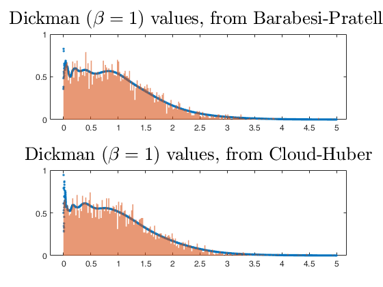
 n Vervaat perpetuity values extracterd with the two implemented methods.
n Vervaat perpetuity values extracterd with the two implemented methods.In the example, we set n = 5000 and \beta = 1.
% The superimposed normal kernel density is just for illustration:
% a more precise density can be simulated with function vervaatxdf.
clear all;
close all
betav = 1;
N = 5000;
y1 = vervaatrnd(betav,N,1);
y2 = vervaatrnd(betav,N,2);
x    = (1:N)*(5*betav)/N;
pd1  = fitdist(y1(:),'Kernel','Kernel','normal','Support','positive');
pdf1 = pdf(pd1,x);
pd2  = fitdist(y2(:),'Kernel','Kernel','normal','Support','positive');
pdf2 = pdf(pd2,x);
figure;
h1 = subplot(2,1,1);
p1h = plot(x,pdf1,'.','LineWidth',2); ylim([0,1]);
if ~verLessThan('matlab','1.7.0')
hold on
h=histogram(y1);
h.Normalization='pdf';
h.BinWidth=0.02;
h.EdgeColor='none';
hold off
end
h2 = subplot(2,1,2);
plot(x,pdf2,'.','LineWidth',2); ylim([0,1]);
if ~verLessThan('matlab','1.7.0')
hold on
h=histogram(y2);
h.Normalization='pdf';
h.BinWidth=0.02;
h.EdgeColor='none';
hold off
end
title(h1,'Dickman ($$\beta = 1 $$) values, from Barabesi-Pratelli' ,'Fontsize',20,'interpreter','latex');
title(h2,'Dickman ($$\beta = 1 $$) values, from Cloud-Huber'       ,'Fontsize',20,'interpreter','latex');
Related Examples
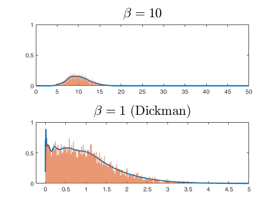
N=5000 random values extracted from two Vervaat perpetuities.
N=5000 random values extracted from two Vervaat perpetuities.Parameters are: \beta = 1 and \beta = 10.
% The superimposed normal kernel density is for illustration:
% a more precise density can be simulated with function vervaatxdf.
close all
clear all;
close all;
betav10 = 10;
betav01 = 1;
N = 5000;
y10 = vervaatrnd(betav10,N);
y01 = vervaatrnd(betav01,N);
pdy10 = fitdist(y10(:),'Kernel','Kernel','normal','Support','positive');
x10   = (1:N)*(5*betav10)/N;
pdf10 = pdf(pdy10,x10);
pdy01 = fitdist(y01(:),'Kernel','Kernel','normal','Support','positive');
x01   = (1:N)*(5*betav01)/N;
pdf01 = pdf(pdy01,x01);
figure;
h1=subplot(2,1,1);
plot(x10,pdf10,'-','LineWidth',2); ylim([0,1]);
if ~verLessThan('matlab','1.7.0')
hold on
h=histogram(y10);
h.Normalization='pdf';
h.BinWidth=0.02;
h.EdgeColor='none';
hold off
end
h2=subplot(2,1,2);
plot(x01,pdf01,'-','LineWidth',2); ylim([0,1]);
if ~verLessThan('matlab','1.7.0')
hold on
h=histogram(y01);
h.Normalization='pdf';
h.BinWidth=0.02;
h.EdgeColor='none';
hold off
end
title(h1,'$$\beta = 10$$' ,'Fontsize',20,'interpreter','latex');
title(h2,'$$\beta = 1 $$ (Dickman)'  ,'Fontsize',20,'interpreter','latex');
Input Arguments
Output Arguments
More About
References
Cloud, K. and Huber, M. (2018), Fast Perfect Simulation of Vervaat Perpetuities, "Journal of Complexity", Vol. 42, pp. 19-30.
Devroye, L. (2001), Simulating perpetuities, "Methodology And Computing In Applied Probability", Vol. 3, Num. 1, pp. 97-115.
Fill, J. A. and Huber, M. (2010), Perfect simulation of Vervaat perpetuities, "Electronic Journal of Probability", Vol. 15, pp. 96-109.
Devroye, L. and Fawzi, O. (2010), Simulating the Dickman distribution, "Statistics and Probability Letters", Vol. 80, pp. 242-247.
Blanchet, J. H. and Sigman, K. (2011), On exact sampling of stochastic perpetuities, "Journal of Applied Probability", Vol. 48A, pp. 165-182.
Takacs, L. (1955), On stochastic processes connected with certain physical recording apparatuses. "Acta Mathematica Academiae Scientificarum Hungarica", Vol. 6, pp 363-379.
Barabesi, L. and Pratelli, L. (2019), On the properties of a Takacs distribution, "Statistics and Probability Letters", Vol. 148, pp. 66-73.