
|
vervaatrnd |
vervaatxdf |
 |
vervaatsim
vervaatsim returns a Vervaat perpetuity.
Syntax
Description
This function allows to simulate exactly from a Vervaat perpetuity distribution with parameter \beta \in (0,+\infty). The simulation method, by K. Cloud, M. Huber (2018), is accurate and very efficient: it is \mathcal{O}(\beta \log(\beta)), in the sense that it uses T uniform random variates, where \mathbf{E}[T] \le \mathcal{O}(\beta \log(\beta)). Therefore the algorithm is good even for \beta \gg 1.
Remark: this function is recursive and cannot be easily extended to the generation of several vervaat numbers.
The FSDA code has been translated from the R version of the authors.
Below we give briefly some definitions, background and motivations. In the references, we also include several key works on the distribution.
Examples
Related Examples
 N=5000 random values extracted from two Vervaat perpetuities.
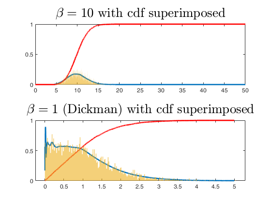
N=5000 random values extracted from two Vervaat perpetuities.Vervaat parameters are: \beta = 1 and \beta = 10.
% The superimposed normal kernel density is just for illustration.
% The same for the superimposed cdf, made using FSDA function exactcdf.
clear all;
close all;
betav10 = 10;
betav01 = 1;
N = 5000;
y10 = zeros(N,1); y01 = y10;
for i=1:N
y10(i) = vervaatsim(betav10);
y01(i) = vervaatsim(betav01);
end
pdy10 = fitdist(y10(:),'Kernel','Kernel','normal','Support','positive');
x10   = (1:N)*(5*betav10)/N;
pdf10 = pdf(pdy10,x10);
pdy01 = fitdist(y01(:),'Kernel','Kernel','normal','Support','positive');
x01   = (1:N)*(5*betav01)/N;
pdf01 = pdf(pdy01,x01);
figure;
h1=subplot(2,1,1);
plot(x10,pdf10,'-','LineWidth',2); ylim([0,1]);
% now superimpose the cdf using function exactcdf
cdf10 = exactcdf(x10,y10);
hold on;
plot(x10,cdf10,'-r','LineWidth',2); ylim([0,1]);
hold off;
% superimpose the histogram
if ~verLessThan('matlab','1.7.0')
hold on
h=histogram(y10);
h.Normalization='pdf';
h.BinWidth=0.02;
h.EdgeColor='none';
hold off
end
drawnow;
h2=subplot(2,1,2);
plot(x01,pdf01,'-','LineWidth',2); ylim([0,1]);
% now superimpose the cdf using function exactcdf
cdf01 = exactcdf(x01,y01);
hold on;
plot(x01,cdf01,'-r','LineWidth',2); ylim([0,1]);
hold off;
% superimpose the histogram
if ~verLessThan('matlab','1.7.0')
hold on
h=histogram(y01);
h.Normalization='pdf';
h.BinWidth=0.02;
h.EdgeColor='none';
hold off
end
drawnow;
title(h1,'$$\beta = 10$$ with cdf superimposed' ,'Fontsize',20,'interpreter','latex');
title(h2,'$$\beta = 1 $$ (Dickman) with cdf superimposed'  ,'Fontsize',20,'interpreter','latex');
Density of Vervaat perpetuity: comparison with original R function.
Density of Vervaat perpetuity: comparison with original R function.
clear all;
close all;
% set common parameters
betav = 1;
steps = 10;
d = 3;
% ensure same random numbers in MATLAB and R
rn = mtR(1);
% Now compute the veervaat in MATLAB
y=vervaatsim(betav,steps,d)
% And finally compute the vervaat in R
disp('To verify coherence of results with the R implementation,');
disp('execute in R the following four lines,');
disp('which allow to replicate the same random numbers;');
disp('then execute the vervaat after sourcing the following R code: ') ;
disp(' ');
disp('NGkind("Mersenne-Twister") #set "Mersenne-Twister" "Inversion"');
disp('set.seed(0) ');
disp('state = .Random.seed ');
disp('runif(1) ');
disp('vervaat(beta = 1,steps = 10,d = 3) ');
disp(' ');
y =

    1.8183

To verify coherence of results with the R implementation,
execute in R the following four lines,
which allow to replicate the same random numbers;
then execute the vervaat after sourcing the following R code:

NGkind("Mersenne-Twister") #set "Mersenne-Twister" "Inversion"
set.seed(0)
state = .Random.seed
runif(1)
vervaat(beta = 1,steps = 10,d = 3)
Input Arguments
Output Arguments
More About
References
Cloud, K. and Huber, M. (2018), Fast Perfect Simulation of Vervaat Perpetuities, "Journal of Complexity", Vol. 42, pp. 19-30.
Devroye, L. (2001), Simulating perpetuities, "Methodology And Computing In Applied Probability", Vol. 3, Num. 1, pp. 97–115.
Fill, J. A. and Huber, M. (2010), Perfect simulation of Vervaat perpetuities, "Electronic Journal of Probability", Vol. 15, pp. 96–109.
Devroye, L. and Fawzi, O. (2010), Simulating the Dickman distribution, "Statistics and Probability Letters", Vol. 80, pp. 242–247.
Blanchet, J. H. and Sigman, K. (2011), On exact sampling of stochastic perpetuities, "Journal of Applied Probability", Vol. 48A, pp. 165–182.
Takacs, L. (1955), On stochastic processes connected with certain physical recording apparatuses. "Acta Mathematica Academiae Scientificarum Hungarica", Vol. 6, pp 363-379.
Barabesi, L. and Pratelli, L. (2019), On the properties of a Takacs distribution, "Statistics and Probability Letters", Vol. 148, pp. 66-73.
See Also
|
|
vervaatrnd |
vervaatxdf |
|
|
|
Functions |
|
• The developers of the toolbox • The forward search group • Terms of Use • Acknowledgments