FSCorAnaeda
FSCorAnaeda performs forward search in correspondence analysis with exploratory data analysis purposes
Description
Examples
 FSCorAnaeda with optional arguments.
FSCorAnaeda with optional arguments.Generate contingency table of size 50-by-5 with total sum of n_ij=2000.
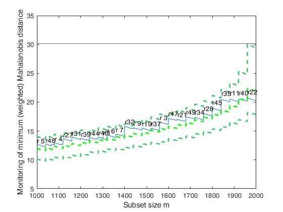
I=50;
J=5;
n=2000;
% nrowt = column vector containing row marginal totals
nrowt=(n/I)*ones(I,1);
% ncolt = row vector containing column marginal totals
ncolt=(n/J)*ones(1,J);
out1=rcontFS(I,J,nrowt,ncolt);
N=out1.m144;
RAW=mcdCorAna(N,'plots',0);
ini=round(sum(sum(RAW.N))/4);
out=FSCorAnaeda(RAW,'plots',1);
Total estimated time to complete MCD:  0.04 seconds
Creating empirical confidence band for minimum (weighted) Mahalanobis distance

Related Examples
Input Arguments
Output Arguments
References
Atkinson, A.C., Riani, M. and Cerioli, A. (2004), "Exploring multivariate data with the forward search", Springer Verlag, New York.