FSMinvmmd

FSMinvmmd converts values of minimum Mahalanobis distance into confidence levels

Syntax

  • mmdinv=FSMinvmmd(mmd,v)example
  • mmdinv=FSMinvmmd(mmd,v,Name,Value)example

Description

example

mmdinv =FSMinvmmd(mmd, v) FSMinvmmd with all default options.

example

mmdinv =FSMinvmmd(mmd, v, Name, Value) FSMinvmmd with optional arguments.

Examples

expand all

  • FSMinvmmd with all default options.
  • After creating 99 per cent confidence envelopes based on 1000 observations and 5 variables are created, their confidence level is calculated with FSMinvmmd.

    v=5;
    mmdenv=FSMenvmmd(1000,v,'prob',0.99);
    mmdinv=FSMinvmmd(mmdenv,v);
    % mmdinv is a matrix which in the second colum contains
    % all values equal to 0.99.

  • FSMinvmmd with optional arguments.
  • Example of finding confidence level of mmd. Forgery Swiss Banknotes data.

    load('swiss_banknotes');
    Y=swiss_banknotes{:,:};
    Y=Y(101:200,:);
    % The line below shows the plot of mmd
    [out]=FSM(Y,'plots',1);
    % The line below transforms the values of mmd into observed confidence
    % levels and shows the output in a plot in normal coordinates using all
    % default options
    plots=struct;
    plots.conflev=[0.01 0.5 0.99 0.999 0.9999 0.99999];
    mmdinv=FSMinvmmd(out.mmd,size(Y,2),'plots',plots);

    Related Examples

    expand all

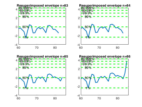
  • Resuperimposing envelopes and normal coordinates.
  • Comparison of resuperimposing envelopes using mmd coordinates and normal coordinates. Forgery Swiss Banknotes data.

    load('swiss_banknotes');
    Y=swiss_banknotes{:,:};
    Y=Y(101:200,:);
    % The line below shows the plot of mmd
    [out]=FSM(Y,'plots',2);
    n0=83:86;
    quantplo=[0.01 0.5 0.99 0.999 0.9999 0.99999];
    ninv=norminv(quantplo);
    lwdenv=2;
    supn0=max(n0);
    ij=0;
    for jn0=n0;
    ij=ij+1;
    MMDinv = FSMinvmmd(out.mmd,size(Y,2),'n',jn0);
    % Resuperimposed envelope in normal coordinates
    subplot(2,2,ij)
    plot(MMDinv(:,1),MMDinv(:,3),'LineWidth',2)
    xlim([out.mmd(1,1) supn0])
    v=axis;
    line(v(1:2)',[ninv;ninv],'color','g','LineWidth',lwdenv,'LineStyle','--','Tag','env');
    text(v(1)*ones(length(quantplo),1),ninv',strcat(num2str(100*quantplo'),'%'));
    title(['Resuperimposed envelope n=' num2str(jn0)]);
    end
    -------------------------
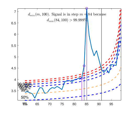
    Signal detection loop
    Tentative signal in central part of the search: step m=84 because
    dmin(84,100)>99.999%
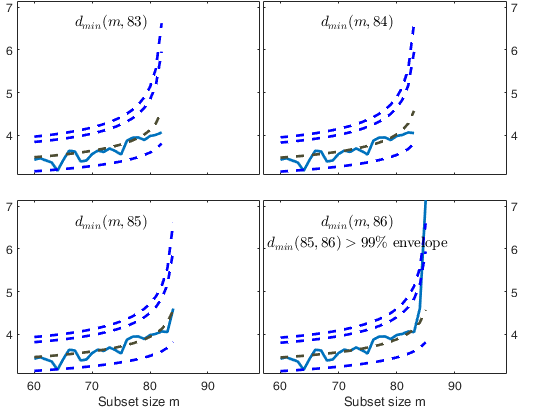
    -------------------
    Signal validation
    Validated signal
    -------------------------------
    Start resuperimposing envelopes from step m=83
    Superimposition stopped because d_{min}(85,86)>99% envelope
    $d_{min}(85,86)>99$\% envelope
    ----------------------------
    Final output
    Number of units declared as outliers=15
    Summary of the exceedances
               1          99         999        9999       99999
               0          21          15           7           7
    
    
    Click here for the graphical output of this example (link to Ro.S.A. website)

    Input Arguments

    expand all

    mmd — Distances. Matrix.

    n-m0 x 2 matrix.

    1st col = fwd search index;

    2nd col = minimum Mahalanobis distance.

    Data Types: single | double

    v — Number of variables. Scalar.

    Number of variables of the underlying dataset.

    Data Types: single | double

    Name-Value Pair Arguments

    Specify optional comma-separated pairs of Name,Value arguments. Name is the argument name and Value is the corresponding value. Name must appear inside single quotes (' '). You can specify several name and value pair arguments in any order as Name1,Value1,...,NameN,ValueN.

    Example: 'n',5 , 'plots',1

    n —It specifies the size of the sample.scalar.

    If it is not specified it is set equal to mmd(end,1)+1.

    Example: 'n',5

    Data Types: double

    plots —Plot on the screen.scalar | structure.

    If plots = 1, a plot which shows the confidence level of mmd in each step is shown on the screen. Three horizontal lines associated respectively with values 0.01, 0.5 and 0.99 are added to the plot.

    If plots is a structure, it may contain the following fields:

    Value Description
    conflev

    vector containing horizontal lines associated with confidence levels;

    conflevlab

    scalar if it is equal 1 labels associated with horizontal lines are shown on the screen;

    xlim

    minimum and maximum on the x axis;

    ylim

    minimum and maximum on the y axis;

    LineWidth

    Line width of the trajectory of mmd in normal coordinates;

    LineStyle

    Line style of the trajectory of mle of transformation parameters;

    LineWidthEnv

    Line width of the horizontal lines;

    Tag

    tag of the plot (default is pl_mmdinv);

    FontSize

    font size of the text labels which identify the trajectories

    Example: 'plots',1

    Data Types: double

    Output Arguments

    expand all

    mmdinv —confidence levels plotted in normal coordinates. (n-m0) -by- 3 matrix (same rows of input matrix mmd)

    It contains information about requested confidence levels plotted in normal coordinates.

    1st col = fwd search index from m0 to n-1;

    2nd col = confidence level of each value of mmd;

    3rd col = confidence level in normal coordinates.

    50 per cent conf level becomes norminv(0.50)=0;

    99 per cent conf level becomes norminv(0.99)=2.33.

    More About

    expand all

    Additional Details

    Let $d^2_i(m )$ and $d_{\mbox{min}}(m)$ be respectively the deletion distance for unit $i$ based on a subset of size $m$ and $d_{\mbox{min}}(m)$ the min. Mahalanobis distance in the forward search at step m. Testing for outliers requires a reference distribution for $d^2_i(m )$ in and hence for $d_{\mbox{min}}(m)$ in (\ref{min}). When $\Sigma$ is estimated from all $n$ observations, the squared statistics have an $F$ distribution.

    However, the estimate $\hat{\Sigma}(m)$ in the search uses the central $m$ out of $n$ observations, so that the variability is underestimated.

    The consistency factor $c(m,n)$ given below

    \[ c(m,n)=\frac{n}{m} C_{v+2} \{C_{v}^{-1} (m/n) \} \]

    where $C_r$ is the c.d.f. of the $\chi^2$ distribution on $r$ degrees of freedom, allows for estimation from this truncated distribution, providing an approximately unbiased estimate of $\Sigma$.

    We can treat the distribution of the rescaled deletion Mahalanobis distance $c(m,n)d_{\mbox{min}}^2(m)$ as a squared deletion distance on $m-1$ degrees of freedom, whose distribution is (Atkinson Riani and Cerioli, 2004; pp. 43-44) \begin{equation}\label{F} \frac{m^2-1}{m(m-v)} F_{v,m-v}, \end{equation} The distribution of the rescaled min Mahalanobis distance $c(m,n) d_{\mbox{min}}^2(m)$ of a subset of size $m$ constructed in such a way that the centroid and covariance matrix of the subset are taken using the units having the $m$ smallest Mahalanobis distances can be treated as the distribution of the $(m+1)$th order statistic from ($F_{v,m-v}$).

    The results of order statistics $Y_{(1)}$, $Y_{(2)}$, $\cdots$, $Y_{(n)}$ from a sample of size $n$ from a distribution with CDF $G(y)$, state that \begin{equation} \label{orderstat} P\{Y_{(m+1)} \le y \} = P \left\{ F_{2(n-m),2(m+1)} > \frac{1-G(y)}{G(y)} \times \frac{m+1}{n-m} \right\} \end{equation} Given that in our case $G(y)$ is the CDF of the $F_{v,m-v}$ we can rewrite this equation as \begin{eqnarray*} && P\{d_{\mbox{ min}}^2(m) \leq \widehat{ d_{\mbox{min}}^2(m)} \} = \\ && 1- F_{2(n-m),2(m+1)} \left( \left( \frac{1}{ F_{v,m-v} \left( \frac{m(m-v)}{m^2-1 } c(m,n) d_{\mbox{min}}^2(m) \right) }-1 \right) \frac{m+1}{n-m} \right) \end{eqnarray*} where $F_{a,b}(y)$ is the CDF of the $F$ distribution with $a$ and $b$ degrees of freedom evaluated in $y$.

    The value of the min. Mahalanobis distance transformed in normal coordinates computed by this routine is nothing but

    \[ \Phi^{-1} \left( P\left\{ d_{\mbox{min}}^2(m) \leq \widehat{ d_{\mbox{min}}^2(m)} \right\} \right) \]

    where $\Phi^{-1}$ is the inverse of the CDF of the standard normal distribution.

    References

    Atkinson, A.C. and Riani, M. (2006), Distribution theory and simulations for tests of outliers in regression, "Journal of Computational and Graphical Statistics", Vol. 15, pp. 460-476.

    Riani, M. and Atkinson, A.C. (2007), Fast calibrations of the forward search for testing multiple outliers in regression, "Advances in Data Analysis and Classification", Vol. 1, pp. 123-141.

    See Also

    | |

    This page has been automatically generated by our routine publishFS