FSRinvmdr
FSRinvmdr converts values of mdr into confidence levels and mdr in normal coordinates
Description
Examples
 FSRinvmdr with optional arguments.
FSRinvmdr with optional arguments.Example of finding confidence level of mdr for untransformed wool data.
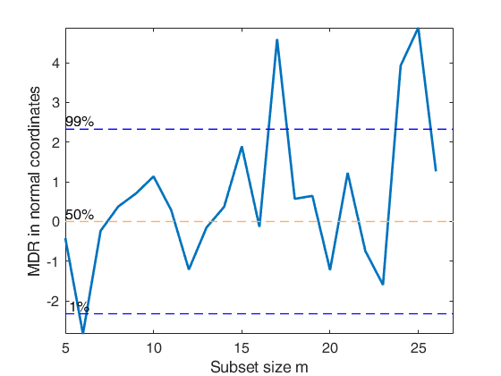
% In the example, the values of mdr are plotted and then transformed
% into observed confidence levels.
% The output is plotted in normal coordinates.
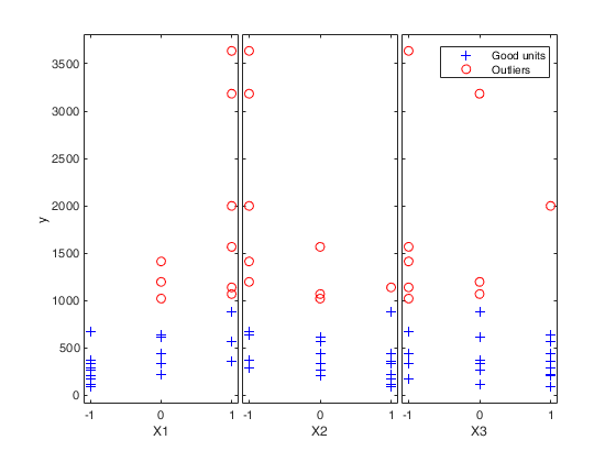
load('wool.txt','wool');
y=wool(:,4);
X=wool(:,1:3);
% The line below shows the plot of mdr
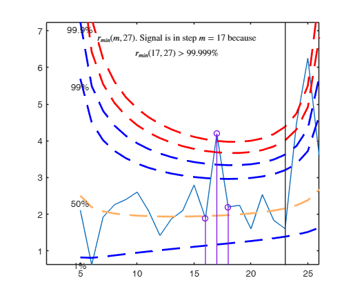
[out]=FSR(y,X,'nsamp',0,'plots',1);
MDRinv=FSRinvmdr(out.mdr,size(X,2)+1,'plots',1);
------------------------------
Warning: Number of subsets without full rank equal to 16.6%
-------------------------
Signal detection loop
Tentative signal in central part of the search: step m=17 because
rmin(17,27)>99.999%

-------------------
Signal validation exceedance of upper envelopes
Validated signal
-------------------------------
Start resuperimposing envelopes from step m=16
Superimposition stopped because r_{min}(17,19)>99% envelope
$r_{min}(17,19)>99$\% envelope
Subsample of 18 units is homogeneous
----------------------------
Final output
Number of units declared as outliers=9
Summary of the exceedances
           1          99         999        9999       99999
           1           3           3           3           2
Related Examples
Input Arguments
Output Arguments
References
Atkinson, A.C. and Riani, M. (2006), Distribution theory and simulations for tests of outliers in regression, "Journal of Computational and Graphical Statistics", Vol. 15, pp. 460-476.
Riani, M. and Atkinson, A.C. (2007), Fast calibrations of the forward search for testing multiple outliers in regression, "Advances in Data Analysis and Classification", Vol. 1, pp. 123-141.