MMregeda
MMregeda computes MM estimator in linear regression for a series of values of efficiency
Syntax
Description
Examples
MMregeda with all default options.
n=200;
p=3;
randn('state', 123456);
X=randn(n,p);
% Uncontaminated data
y=randn(n,1);
% Contaminated data
ycont=y;
ycont(1:5)=ycont(1:5)+6;
[out]=MMregeda(ycont,X);
MMregeda with optional input arguments.
MMregeda using the optimal rho function
n=200;
p=3;
randn('state', 123456);
X=randn(n,p);
% Uncontaminated data
y=randn(n,1);
% Contaminated data
ycont=y;
ycont(1:5)=ycont(1:5)+6;
[out]=MMregeda(ycont,X,'Srhofunc','optimal','rhofunc','optimal');
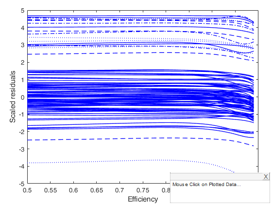
 Comparing the output of different MMreg runs.
Comparing the output of different MMreg runs.
state=100;
randn('state', state);
n=100;
X=randn(n,3);
bet=[3;4;5];
y=3*randn(n,1)+X*bet;
y(1:20)=y(1:20)+13;
%For outlier detection we consider both the nominal individual 1%
%significance level and the simultaneous Bonferroni confidence level.
% Define nominal confidence level
conflev=[0.99,1-0.01/length(y)];
% Define number of subsets
nsamp=3000;
% MM estimators
[out]=MMregeda(y,X,'conflev',conflev(1));
laby='Scaled MM residuals';
resfwdplot(out)
Total estimated time to complete S estimate: 0.03 seconds
Input Arguments
y — Response variable.
Vector.
A vector with n elements that contains the response variable. y can be either a row or a column vector.
Data Types: single| double
X — Data matrix of explanatory variables (also called 'regressors') of
dimension (n x p-1).
Rows of X represent observations, and columns
represent variables.
Missing values (NaN's) and infinite values (Inf's) are allowed, since observations (rows) with missing or infinite values will automatically be excluded from the computations.
Data Types: single| double
Name-Value Pair Arguments
Specify optional comma-separated pairs of Name,Value arguments.
Name is the argument name and Value
is the corresponding value. Name must appear
inside single quotes (' ').
You can specify several name and value pair arguments in any order as
Name1,Value1,...,NameN,ValueN.
 'conflev',0.99
, 'covrob',3
, 'eff',[0.85 0.90 0.95 0.99]
, 'effshape',1
, 'InitialEst',[]
, 'intercept',false
, 'msg',false
, 'nocheck',true
, 'refsteps',10
, 'rhofunc','optimal'
, 'rhofuncparam',5
, 'Snsamp',1000
, 'tol',1e-10
, 'plots',0
conflev
—Confidence level which is
used to declare units as outliers.scalar.
Usually conflev=0.95, 0.975 0.99 (individual alpha) or 1-0.05/n, 1-0.025/n, 1-0.01/n (simultaneous alpha).
Default value is 0.975
Example: 'conflev',0.99
Data Types: double
covrob
—scalar.a number in the set 0, 1, .
.., 5 which specifies the type of covariance matrix of robust beta coefficients.
These numbers correspond to estimators covrob, covrob1, covrob2, covrob4, covrob4 and covrobc detailed inside file RobCov. The default value is 5 (i.e. estimator covrobc).
Example: 'covrob',3
Data Types: single | double
eff
—nominal efficiency.scalar | vector.
Vector defining nominal efficiency (i.e. a series of numbers between 0.5 and 0.99). The default value is the sequence 0.5:0.01:0.99 Asymptotic nominal efficiency is: $(\int \psi' d\Phi)^2 / (\psi^2 d\Phi)$
Example: 'eff',[0.85 0.90 0.95 0.99]
Data Types: double
effshape
—location or scale efficiency.dummy scalar.
If effshape=1, efficiency refers to shape efficiency, else (default) efficiency refers to location.
Example: 'effshape',1
Data Types: double
InitialEst
—starting values of the MM-estimator.[] (default) | structure.
InitialEst must contain the following fields:
| Value | Description |
|---|---|
beta |
v x 1 vector (estimate of the initial regression coefficients) |
scale |
scalar (estimate of the scale parameter). If InitialEst is empty (default) or InitialEst.beta contains NaN values, program uses S estimators. In this last case, it is possible to specify the options given in function Sreg. |
Example: 'InitialEst',[]
Data Types: struct or empty value
intercept
—Indicator for constant term.true (default) | false.
Indicator for the constant term (intercept) in the fit, specified as the comma-separated pair consisting of 'Intercept' and either true to include or false to remove the constant term from the model.
Example: 'intercept',false
Data Types: boolean
msg
—Level of output to display.boolean.
It controls whether to display or not messages on the screen.
If msg==true (default), messages are displayed on the screen about estimated time to compute the initial S estimator and the warnings about 'MATLAB:rankDeficientMatrix', 'MATLAB:singularMatrix' and 'MATLAB:nearlySingularMatrix' are set to off.
If msg is false, no message is displayed on the screen.
Example: 'msg',false
Data Types: logical
nocheck
—Check input arguments.boolean.
If nocheck is equal to true, no check is performed on matrix y and matrix X. Notice that y and X are left unchanged. In other words, the additional column of ones for the intercept is not added.
As default nocheck=false.
Example: 'nocheck',true
Data Types: boolean
refsteps
—Maximum iterations.scalar.
Scalar defining maximum number of iterations in the MM loop. Default value is 100.
Example: 'refsteps',10
Data Types: double
rhofunc
—rho function.string.
String which specifies the rho function which must be used to weight the residuals in MM step.
Possible values are: 'bisquare';
'optimal';
'hyperbolic';
'hampel';
'mdpd';
'AS'.
'bisquare' uses Tukey's $\rho$ and $\psi$ functions.
See TBrho and TBpsi.
'optimal' uses optimal $\rho$ and $\psi$ functions.
See OPTrho and OPTpsi.
'hyperbolic' uses hyperbolic $\rho$ and $\psi$ functions.
See HYPrho and HYPpsi.
'hampel' uses Hampel $\rho$ and $\psi$ functions.
See HArho and HApsi.
'mdpd' uses Minimum Density Power Divergence $\rho$ and $\psi$ functions.
'AS' uses Andrew's sine $\rho$ and $\psi$ functions.
The default is bisquare.
Example: 'rhofunc','optimal'
Data Types: char
rhofuncparam
—Additional parameters for the specified rho function in the MM step.scalar | vector.
For hyperbolic rho function it is possible to set up the value of k = sup CVC (the default value of k is 4.5).
For Hampel rho function it is possible to define parameters a, b and c (the default values are a=2, b=4, c=8).
Example: 'rhofuncparam',5
Data Types: single | double
Soptions
—options if initial estimator is S and InitialEst is empty.sbestr, Sminsctol, Srhofunc, Smsg, Snsamp, Srefsteps, Sreftol, Srefstepsbestr, Sreftolbestr.
See function Sreg for more details on these options.
It is necessary to add to the S options the letter S at the beginning. For example, if you want to use the optimal rho function the supplied option is 'Srhofunc','optimal'. For example, if you want to use 3000 subsets, the supplied option is 'Snsamp',3000.
Note that the rho function which is used in the MMstep is the same as the one used in the S step.
Example: 'Snsamp',1000
Data Types: single | double
tol
—Tolerance.scalar.
Scalar controlling tolerance in the MM loop.
Default value is 1e-7.
Example: 'tol',1e-10
Data Types: double
plots
—Plot on the screen.scalar | structure.
If plots = 1, generates a plot with the robust residuals against index number. The confidence level used to draw the confidence bands for the residuals is given by the input option conflev. If conflev is not specified, a nominal 0.975 confidence interval will be used.
Example: 'plots',0
Data Types: single | double
Output Arguments
out — description
Structure
A structure containing the following fields:
| Value | Description |
|---|---|
auxscale |
scalar, S estimate of the scale (or supplied external estimate of scale, if option InitialEst is not empty). |
Beta |
matrix of size length(eff)-by-(p+1) containing the S estimator of regression coefficients for each value of eff. The first column contains the value of eff. |
tStat |
matrix of size length(eff)-by-(p+1) containing the MM estimator of t statistics for each value of eff. The first column contains the value of eff. |
RES |
n x length(eff) matrix containing scaled MM residuals for each value of eff. out.RES(:,jj)=(y-X*out.Beta(:,jj))/out.auxscale |
Weights |
n x length(eff) matrix. Weights assigned to each observation for each value of eff. |
Outliers |
n x length(eff) Boolean matrix containing the outliers which have been found for each value of eff. |
Sbeta |
p x 1 vector containing S estimate of regression coefficients (or supplied initial external estimate of regression coefficients, if option InitialEst is not empty). |
Ssingsub |
Number of subsets without full rank in the S preliminary part. Notice that out.singsub > 0.1*(number of subsamples) produces a warning. |
conflev |
Confidence level that was used to declare outliers. |
rhofunc |
string identifying the rho function which has been used. |
rhofuncparam |
vector which contains the additional parameters for the specified rho function that have been used. For hyperbolic rho function the value of k =sup CVC. For Hampel rho function the parameters a, b and c. out.Outliers = Boolean matrix containing the list of the units declared as outliers for each value of eff using confidence level specified in input scalar conflev. |
eff |
vector containing the value of eff which have been used. out.Sbeta = vector. S initial estimate of regression coefficients. |
y |
response vector y. |
X |
Data matrix of explanatory variables which has been used (it also contains the column of ones if input option intercept was missing or equal to 1). |
class |
'MMregeda'. |
References
Riani, M., Cerioli, A., Atkinson, A.C. and Perrotta, D. (2014), Monitoring Robust Regression, "Electronic Journal of Statistics", Vol. 8, pp. 646-677.
Maronna, R.A., Martin D. and Yohai V.J. (2006), "Robust Statistics, Theory and Methods", Wiley, New York.
Acknowledgements