RobCov

robCov computes covariance matrix of robust regression coefficients

Syntax

  • out=RobCov(X,scaledres,scaleest)example
  • out=RobCov(X,scaledres,scaleest,Name,Value)example

Description

Under some regularity conditions, robust (S and MM) estimates are asymptotically normal, thereby allowing for Wald-type tests and confidence intervals. The covariance matrix of the estimated parameters \[ cov(\hat \beta)= q^2 \times \sigma^2 \times v \times V_X^{-1} \]

consists of four parts: 1) $q$ a correction factor for the scale estimate;

2) $\sigma$ the scale parameter.

3) $v$ a correction factor depending on the $\psi$ function which is used;

4) $V_X$= a matrix part. For OLS $V_X=X'X$. Given that in robust regression we give a weight to each observation, the matrix $X'X$ should be replaced by something like $X'WX$, where $W$ is a diagonal matrix containing the weights assigned to each observation.

The purpose of this function is to provide the user with different options for the estimate of $cov(\hat \beta)$ where $\hat \beta$ is a vector of regression coefficients obtained using S or MM estimation and a particular $\rho$ function.

example

out =RobCov(X, scaledres, scaleest) Compare the 5 estimates of cov matrix.

example

out =RobCov(X, scaledres, scaleest, Name, Value) Compare t stat from S and MM estimator.

Examples

expand all

  • Compare the 5 estimates of cov matrix.
  • n=200;
    p=3;
    state1=123456;
    randn('state', state1);
    X=randn(n,p);
    y=randn(n,1);
    kk=10;
    ycont = y;
    ycont(1:kk)=ycont(1:kk)+7;
    [outS]=Sreg(ycont,X);
    rhofunc='optimal';
    bdp=0.5;
    out=RobCov(X,outS.residuals,outS.scale);
    disp('Compare 5 estimates of cov(\hat beta)')
    disp('covrob'); disp(out.covrob)
    disp('--------')
    disp('covrob1'); disp(out.covrob1)
    disp('--------')
    disp('covrob2'); disp(out.covrob2)
    disp('--------')
    disp('covrob3'); disp(out.covrob3)
    disp('--------')
    disp('covrob4'); disp(out.covrob4)
    disp('--------')
    disp('covrobc'); disp(out.covrobc)

  • Compare t stat from S and MM estimator.
  • n=200;
    p=3;
    state1=123456;
    randn('state', state1);
    X=randn(n,p);
    y=randn(n,1);
    kk=10;
    ycont = y;
    ycont(1:kk)=ycont(1:kk)+7;
    [outS]=Sreg(ycont,X);
    rhofunc='optimal';
    bdp=0.5;
    out=RobCov(X,outS.residuals,outS.scale,'rhofunc',rhofunc,'bdp',0.5);
    covrobS=out.covrob;
    covrobS1=out.covrob1;
    covrobS2=out.covrob2;
    covrobS3=out.covrob3;
    covrobS4=out.covrob4;
    % Compute robust S t-statistics
    tstatS=outS.beta./sqrt(diag(covrobS));
    tstatS1=outS.beta./sqrt(diag(covrobS1));
    tstatS2=outS.beta./sqrt(diag(covrobS2));
    tstatS3=outS.beta./sqrt(diag(covrobS3));
    tstatS4=outS.beta./sqrt(diag(covrobS4));
    eff=0.95;
    outMM=MMregcore(ycont,X,outS.beta,outS.scale);
    out=RobCov(X,outMM.residuals,outS.scale,'rhofunc',rhofunc,'eff',eff);
    covrobMM=out.covrob;
    covrobMM1=out.covrob1;
    covrobMM2=out.covrob2;
    covrobMM3=out.covrob3;
    covrobMM4=out.covrob4;
    tstatMM=outMM.beta./sqrt(diag(covrobMM));
    tstatMM1=outMM.beta./sqrt(diag(covrobMM1));
    tstatMM2=outMM.beta./sqrt(diag(covrobMM2));
    tstatMM3=outMM.beta./sqrt(diag(covrobMM3));
    tstatMM4=outMM.beta./sqrt(diag(covrobMM4));
    disp('tstat from S')
    disp([tstatS tstatS1 tstatS2 tstatS3 tstatS4])
    disp('--------')
    disp('tstat from MM')
    disp([tstatMM tstatMM1 tstatMM2 tstatMM3 tstatMM4])
    qhat=out.q;
    disp('tstat from MM after correction for sigma')
    disp([tstatMM/qhat tstatMM1/qhat tstatMM2/qhat tstatMM3/qhat tstatMM4/qhat])

    Related Examples

    expand all

  • An example of the need of using covrobc.
  • XX is a 50-by-2 matrix generated by standard random normal.

    % Estimate beta using Sreg and compare the four estimators of 
    % cov (\hat \beta).
    XX=[0.8115    1.3104
    -0.4477    0.8110
    0.9438    1.9121
    -0.2346    0.7058
    1.8364    3.1318
    0.2911    0.7837
    0.3669    1.7571
    0.4560    1.0876
    -1.0831    0.0679
    0.7018    1.0923
    1.6976    2.7744
    -0.0624    1.2015
    0.2016    0.7747
    -0.1542    1.3095
    -0.9416   -0.5251
    0.4873    0.8116
    -0.3561    0.9261
    0.5185    2.1219
    -0.7674   -0.0514
    0.3360    1.8620
    -0.2083    1.3796
    -0.1700    0.9053
    1.9152    2.4369
    -0.9912   -0.6885
    0.5939    2.0449
    -1.1842   -0.8506
    1.1375    1.6184
    -0.2482    1.2104
    0.7936    2.2313
    -0.2744    1.5259
    1.1455    2.2739
    -0.0637    1.2618
    -0.5054    0.0536
    0.7282    1.9411
    -0.0703    0.8090
    -1.8186   -0.8725
    -2.0621   -0.5299
    -1.7750   -0.7765
    -0.8553   -0.3311
    1.8966    2.9885
    -0.1076    0.5106
    0.9055    1.1283
    0.3086    1.5491
    -0.0487    0.4964
    -1.6901   -0.7348
    -0.7253    0.9436
    0.2124    0.6549
    -0.2748   -0.2009
    -1.2804   -0.7036
    0.3627    1.3027];
    % Define X and y;
    y=XX(:,2);
    X=XX(:,1);
    outS=Sreg(y,X,'rhofunc','bisquare','bdp',0.5);
    out=RobCov(X,outS.residuals,1,'rhofunc','bisquare','bdp',0.5);
    disp('covrob'); disp(out.covrob)
    disp('--------')
    disp('covrob1'); disp(out.covrob1)
    disp('--------')
    disp('covrob2'); disp(out.covrob2)
    disp('--------')
    disp('covrob3'); disp(out.covrob3)
    disp('--------')
    disp('covrob4'); disp(out.covrob4)
    disp('--------')
    disp('covrobc'); disp(out.covrobc)
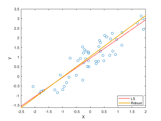
    % plot X and y and add LS and robust regression line
    plot(X,y,'o')
    xlabel('X')
    ylabel('y')
    hLS=lsline;
    hLS.Color='r';
    hLS.LineStyle = ':';
    hLS.LineWidth = 2;
    hROB=refline([outS.beta(2) outS.beta(1)]);
    hROB.LineWidth = 2;
    legend({'' 'LS','Robust'},'Location','Best')
    Total estimated time to complete S estimate:  0.69 seconds 
    covrob
        0.6426   -0.0036
       -0.0036    0.7248
    
    --------
    covrob1
       29.6355   -0.4573
       -0.4573   29.4373
    
    --------
    covrob2
       29.6292   -0.1654
       -0.1654   33.4196
    
    --------
    covrob3
        0.2391   -0.0037
       -0.0037    0.2375
    
    --------
    covrob4
       1.0e-03 *
    
        0.2843   -0.0069
       -0.0069    0.2487
    
    --------
    covrobc
        0.6426   -0.0036
       -0.0036    0.7248
    
    
    Click here for the graphical output of this example (link to Ro.S.A. website)

    Input Arguments

    expand all

    X — Data matrix of explanatory variables (also called 'regressors') of dimension (n x p-1). Rows of X represent observations, and columns represent variables.

    Data Types: single | double

    scaledres — Scaled residuals.Vector. n-times-1 vector containing scaled residuals $r_i/\hat \sigma$.

    Data Types: single | double

    scaleest — robust estimate of the scale. Scalar.

    Robust estimate of sigma ($\hat \sigma$).

    Data Types: single | double

    Name-Value Pair Arguments

    Specify optional comma-separated pairs of Name,Value arguments. Name is the argument name and Value is the corresponding value. Name must appear inside single quotes (' '). You can specify several name and value pair arguments in any order as Name1,Value1,...,NameN,ValueN.

    Example: 'intercept',false , 'eff',0.99 , 'bdp',0.4 , 'rhofunc','optimal' , 'rhofuncparam',5

    intercept —Indicator for constant term.true (default) | false.

    Indicator for the constant term (intercept) in the fit, specified as the comma-separated pair consisting of 'Intercept' and either true to include or false to remove the constant term from the model.

    Example: 'intercept',false

    Data Types: boolean

    eff —nominal efficiency.scalar.

    Scalar defining nominal efficiency (i.e. a number between 0.5 and 0.99). The default value is 0.95 Asymptotic nominal efficiency is: $(\int \psi' d\Phi)^2 / (\psi^2 d\Phi)$

    Example: 'eff',0.99

    Data Types: double

    bdp —breakdown point.scalar.

    It measures the fraction of outliers the algorithm should resist. In this case any value greater than 0 but smaller or equal than 0.5 will do fine.

    Note that given bdp nominal efficiency is automatically determined.

    REMARK: just one between bdp and eff must be specified. If both of them are specified an error is produced. If both of them are not specified the defulat is tu use the tuning constant associated to a nominal efficiency of 0.95.

    Example: 'bdp',0.4

    Data Types: double

    rhofunc —rho function.string.

    String which specifies the rho function which must be used to weight the residuals.

    Possible values are 'bisquare' 'optimal' 'hyperbolic' 'hampel'.

    'bisquare' uses Tukey's $\rho$ and $\psi$ functions.

    See TBrho and TBpsi.

    'optimal' uses optimal $\rho$ and $\psi$ functions.

    See OPTrho and OPTpsi.

    'hyperbolic' uses hyperbolic $\rho$ and $\psi$ functions.

    See HYPrho and HYPpsi.

    'hampel' uses Hampel $\rho$ and $\psi$ functions.

    See HArho and HApsi.

    'mdpd' uses Minimum Density Power Divergence $\rho$ and $\psi$ functions.

    See PDrho and PDpsi.

    'AS' uses Andrews' sine $\rho$ and $\psi$ functions.

    See ASrho and ASpsi.

    The default is bisquare

    Example: 'rhofunc','optimal'

    Data Types: double

    rhofuncparam —Additional parameters for the specified rho function.scalar | vector.

    For hyperbolic rho function it is possible to set up the value of k = sup CVC (the default value of k is 4.5).

    For Hampel rho function it is possible to define parameters a, b and c (the default values are a=2, b=4, c=8)

    Example: 'rhofuncparam',5

    Data Types: single | double

    Output Arguments

    expand all

    out — description Structure

    A structure containing the following fields

    Value Description
    covrob

    p-times-p (if intercept is true else is (p-1)-by-(p-1)) matrix containing asymptotic variance covariance matrix of regression coefficients. covrob uses equation (4.49) of p. 101 of Maronna et al. (2006) namely: \[ \mbox{covrob} = cov( \hat \beta) = \hat \sigma^2 \hat v (X'X)^{-1} \] where \[ \hat v = \frac{n}{n-p} n\frac{\sum_{i=1}^n \psi(r_i/\hat \sigma)^2}{[\sum_{i=1}^n \psi'(r_i/\hat \sigma)]^2} \]

    covrob1

    p-times-p (if intercept is true else is (p-1)-by-(p-1)) matrix containing asymptotic variance covariance matrix of regression coefficients. covrob1 uses equation (7.81) of p. 171 of Huber and Ronchetti (2009) with $(X'X)^{-1}$ replaced by $(X' W X)^{-1}$ namely: \[ \mbox{covrob1} = K^2 \hat v (X' W X)^{-1}; \] where $K=1+\frac{p}{n} \frac{var(\psi' (r/\hat \sigma))}{ \left[ \sum_{i=1}^n \psi'(r_i/\hat \sigma)/n \right]^2}= 1+[CV(\psi')]^2 p/n $. The notation $CV(\psi')$ stands for the coefficient of variation of $\psi'$, where $\psi$ and $\psi'$ are, respectively, the first and second derivatives of the $\rho$ function.

    covrob2

    p-times-p (if intercept is true else is (p-1)-by-(p-1)) matrix containing asymptotic variance covariance matrix of regression coefficients. covrob2 uses equation (7.81) of p. 171 of Huber and Ronchetti (2009) with $X'X$ and $K^2$ namely: \[ \mbox{covrob2} = K^2 \hat v (X' X)^{-1}; \]

    covrob3

    p-times-p (if intercept is true else is (p-1)-by-(p-1)) matrix containing asymptotic variance covariance matrix of regression coefficients. covrob uses equation (7.82) of p. 171 of Huber and Ronchetti (2009).

    namely:

    \[ \mbox{covrob3} = K \frac{n}{n-p} \frac{\sum_{i=1}^n \psi (r_i/\hat \sigma)^2}{\sum_{i=1}^n \psi'(r_i/\hat \sigma)} (X' W X)^{-1}; \]

    covrob4

    p-times-p (if intercept is true else is (p-1)-by-(p-1)) matrix containing asymptotic variance covariance matrix of regression coefficients. covrob4 uses equation (7.83) of p. 171 of of Huber and Ronchetti (2009).

    namely:

    \[ \mbox{covrob4} = \frac{1}{n-p} K^{-1} \sum_{i=1}^n \psi(r_i/\hat \sigma)^2 (X' W X)^{-1} X'X (X' W X)^{-1}; \]

    covrobc

    p-times-p (if intercept is true else is (p-1)-by-(p-1)) matrix containing best variance covariance matrix of regression coefficients. covrobc checks the coefficient of variation of the derivative of function $\psi(r_i/\hat \sigma)$. If it is greater than the threshold proposed in Salini, et al. (2020), it uses covrob else covrob2.

    q

    scalar. Correction for scale estimate (see Maronna and Yohai CSDA 2010). It is defined as \[ q=1+\frac{p}{2n} \frac{a}{b \times c} \] where \[ a = \frac{1}{n} \sum_{i=1}^n \psi(r_i/\hat \sigma)^2 \] \[ b = \frac{1}{n} \sum_{i=1}^n \psi'(r_i/\hat \sigma) \] \[ c = \frac{1}{n} \sum_{i=1}^n \psi(r_i/\hat \sigma) r_i/\hat \sigma \]

    References

    Maronna, R.A., Martin D. and Yohai V.J. (2006), "Robust Statistics, Theory and Methods", Wiley, New York.

    Huber, P.J. and Ronchetti, E.M. (2009), "Robust Statistics, 2nd Edition", Wiley.

    Maronna, R.A., and Yohai V.J. (2010), Correcting MM estimates for fat data sets, "Computational Statistics and Data Analysis", Vol. 54, pp. 3168-3173.

    Koller, M. and W. A. Stahel (2011), Sharpening wald-type inference in robust regression for small samples, "Computational Statistics & Data Analysis", Vol. 55, pp. 2504-2515.

    Croux, C., Dhaene G., and Hoorelbeke D. (2003), Robust standard errors for robust estimators. Technical report, Dept. of Applied Economics, KU Leuven.

    Salini, S., Laurini, F., Morelli, G., Riani M. and Cerioli A. (2022), Covariance matrices of S robust regression estimators, Journal of Statistical Computation and Simulation, Vol. 92, pp. 724-747, https://doi.org/10.1080/00949655.2021.1972300

    See Also

    | |

    This page has been automatically generated by our routine publishFS