Taureg

Taureg computes Tau estimators in linear regression

Syntax

Description

example

out =Taureg(y, X) Taureg with all default options.

example

out =Taureg(y, X, Name, Value) Taureg with optional arguments.

example

[out , varargout] =Taureg(___) Taureg with optimal rho function.

Examples

expand all

  • Taureg with all default options.
  • n=200;
    p=3;
    rng('default')
    randn('state', 123456);
    X=randn(n,p);
    % Uncontaminated data
    y=randn(n,1);
    % Contaminated data
    ycont=y;
    ycont(1:5)=ycont(1:5)+6;
    [out]=Taureg(ycont,X);

  • Taureg with optional arguments.
  • n=200;
    p=3;
    randn('state', 123456);
    X=randn(n,p);
    % Uncontaminated data
    y=randn(n,1);
    % Contaminated data
    ycont=y;
    ycont(1:5)=ycont(1:5)+6;
    [out]=Taureg(ycont,X,'plots',1);
    Warning: Using 'state' to set RANDN's internal state causes RAND, RANDI, and
    RANDN to use legacy random number generators.  This syntax is not recommended.
    See <a href="matlab:helpview([docroot '\techdoc\math\math.map'],'update_random_number_generator')">Replace Discouraged Syntaxes of rand and randn</a> to use RNG to replace the
    old syntax. 
    Total estimated time to complete tau estimate:  1.73 seconds 
    
    Click here for the graphical output of this example (link to Ro.S.A. website).

  • Taureg with optimal rho function.
  • n=200;
    p=3;
    randn('state', 123456);
    X=randn(n,p);
    % Uncontaminated data
    y=randn(n,1);
    % Contaminated data
    ycont=y;
    ycont(1:5)=ycont(1:5)+6;
    [out]=Taureg(ycont,X,'plots',1,'rhofunc','optimal');

    Related Examples

    expand all

  • Taureg with hyperbolic rho function.
  • n=200;
    p=3;
    randn('state', 123456);
    X=randn(n,p);
    % Uncontaminated data
    y=randn(n,1);
    % Contaminated data
    ycont=y;
    ycont(1:5)=ycont(1:5)+6;
    [out]=Taureg(ycont,X,'plots',1,'rhofunc','hyperbolic');

  • Taureg with Hampel rho function.
  • With parameters a=1.5 b=3.5 c=8.

    n=200;
    p=3;
    randn('state', 123456);
    X=randn(n,p);
    % Uncontaminated data
    y=randn(n,1);
    % Contaminated data
    ycont=y;
    ycont(1:5)=ycont(1:5)+6;
    rhofuncparam=[1.5 3.5 8];
    [out]=Taureg(ycont,X,'plots',1,'rhofunc','hampel','rhofuncparam',rhofuncparam);

  • Taureg: comparison between bisquare, power divergence and Andrew's sine rho function.
  • n=200;
    p=3;
    close all
    rng('default')
    rng(123456)
    X=randn(n,p);
    % Uncontaminated data
    y=randn(n,1);
    % Contaminated data
    ycont=y;
    ycont(1:5)=ycont(1:5)+6;
    [out]=Taureg(ycont,X,'plots',0,'rhofunc','bisquare');
    h1=subplot(3,1,1);
    resindexplot(out,'h',h1)
    title('Tukey''s bisquare rho function')
    [out]=Taureg(ycont,X,'plots',0,'rhofunc','mdpd');
    h2=subplot(3,1,2);
    resindexplot(out,'h',h2)
    title('Power divergence rho function')
    Total estimated time to complete tau estimate:  0.87 seconds 
    Total estimated time to complete tau estimate:  0.28 seconds 
    
    Click here for the graphical output of this example (link to Ro.S.A. website)

    Input Arguments

    expand all

    y — Response variable. Vector.

    A vector with n elements that contains the response variable. y can be either a row or a column vector.

    Data Types: single| double

    X — Data matrix of explanatory variables (also called 'regressors') of dimension (n x p-1). Rows of X represent observations, and columns represent variables.

    Missing values (NaN's) and infinite values (Inf's) are allowed, since observations (rows) with missing or infinite values will automatically be excluded from the computations.

    Data Types: single| double

    Name-Value Pair Arguments

    Specify optional comma-separated pairs of Name,Value arguments. Name is the argument name and Value is the corresponding value. Name must appear inside single quotes (' '). You can specify several name and value pair arguments in any order as Name1,Value1,...,NameN,ValueN.

    Example: 'intercept',false , 'bdp',0.4 , 'eff',0.99 , 'rhofunc','optimal' , 'rhofuncparam',5 , 'nsamp',1000 , 'nsamp',1000 , 'nsamp',1000 , 'refstepsbestr',10 , 'reftolbestr',1e-10 , 'minsctol',1e-7 , 'bestr',10 , 'conflev',0.99 , 'msg',0 , 'nocheck',true , 'plots',0 , 'yxsave',1

    intercept —Indicator for constant term.true (default) | false.

    Indicator for the constant term (intercept) in the fit, specified as the comma-separated pair consisting of 'Intercept' and either true to include or false to remove the constant term from the model.

    Example: 'intercept',false

    Data Types: boolean

    bdp —breakdown point.scalar.

    It measures the fraction of outliers the algorithm should resist. In this case any value greater than 0 but smaller or equal than 0.5 will do fine (default=0.5).

    Note that given bdp nominal efficiency is automatically determined.

    Example: 'bdp',0.4

    Data Types: double

    eff —nominal efficiency.scalar.

    Scalar defining nominal efficiency (i.e. a number between 0.5 and 0.99). The default value is 0.95 Asymptotic nominal efficiency is:

    Example: 'eff',0.99

    Data Types: double

    rhofunc —rho function.string.

    String which specifies the rho function which must be used to weight the residuals.

    Possible values are 'bisquare' 'optimal' 'hyperbolic' 'hampel' 'mdpd';

    'AS'.

    'bisquare' uses Tukey's $\rho$ and $\psi$ functions.

    See TBrho and TBpsi.

    'optimal' uses optimal $\rho$ and $\psi$ functions.

    See OPTrho and OPTpsi.

    'hyperbolic' uses hyperbolic $\rho$ and $\psi$ functions.

    See HYPrho and HYPpsi.

    'hampel' uses Hampel $\rho$ and $\psi$ functions.

    See HArho and HApsi.

    'mdpd' uses Minimum Density Power Divergence $\rho$ and $\psi$ functions.

    See PDrho and PDpsi.

    'AS' uses Andrew's sine $\rho$ and $\psi$ functions.

    See ASrho and ASpsi.

    The default is bisquare

    Example: 'rhofunc','optimal'

    Data Types: character

    rhofuncparam —Additional parameters for the specified rho function.scalar | vector.

    For hyperbolic rho function it is possible to set up the value of k = sup CVC (the default value of k is 4.5).

    For Hampel rho function it is possible to define parameters a, b and c (the default values are a=2, b=4, c=8)

    Example: 'rhofuncparam',5

    Data Types: single | double

    nsamp —Number of subsamples which will be extracted to find the robust estimator.scalar.

    If nsamp=0 all subsets will be extracted.

    They will be (n choose p).

    If the number of all possible subset is <1000 the default is to extract all subsets otherwise just 1000.

    Example: 'nsamp',1000

    Data Types: single | double

    refsteps —Number of refining iterations.scalar.

    Number of refining iterationsin each subsample (default = 3).

    refsteps = 0 means "raw-subsampling" without iterations.

    Example: 'nsamp',1000

    Data Types: single | double

    reftol —scalar.default value of tolerance for the refining steps.

    The default value is 1e-6;

    Example: 'nsamp',1000

    Data Types: single | double

    refstepsbestr —number of refining iterations for each best subset.scalar.

    Scalar defining number of refining iterations for each best subset (default = 50).

    Example: 'refstepsbestr',10

    Data Types: single | double

    reftolbestr —Tolerance for the refining steps.scalar.

    Tolerance for the refining steps for each of the best subsets The default value is 1e-8;

    Example: 'reftolbestr',1e-10

    Data Types: single | double

    minsctol —tolerance for the iterative procedure for finding the minimum value of the scale.scalar.

    Value of tolerance for the iterative procedure for finding the minimum value of the scale for each subset and each of the best subsets (It is used by subroutine minscale.m) The default value is 1e-7;

    Example: 'minsctol',1e-7

    Data Types: single | double

    bestr —number of "best betas" to remember.scalar.

    Scalar defining number of "best betas" to remember from the subsamples. These will be later iterated until convergence (default=5)

    Example: 'bestr',10

    Data Types: single | double

    conflev —Confidence level which is used to declare units as outliers.scalar.

    Usually conflev=0.95, 0.975 0.99 (individual alpha) or 1-0.05/n, 1-0.025/n, 1-0.01/n (simultaneous alpha).

    Default value is 0.975

    Example: 'conflev',0.99

    Data Types: double

    msg —Level of output to display.scalar.

    It controls whether to display or not messages on the screen.

    If msg==1 (default) messages are displayed on the screen about estimated time to compute the estimator and the warnings about 'MATLAB:rankDeficientMatrix', 'MATLAB:singularMatrix' and 'MATLAB:nearlySingularMatrix' are set to off else no message is displayed on the screen

    Example: 'msg',0

    Data Types: single | double

    nocheck —Check input arguments.boolean.

    If nocheck is equal to true no check is performed on matrix y and matrix X. Notice that y and X are left unchanged. In other words the additional column of ones for the intercept is not added.

    As default nocheck=false.

    Example: 'nocheck',true

    Data Types: boolean

    plots —Plot on the screen.scalar | structure.

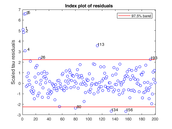
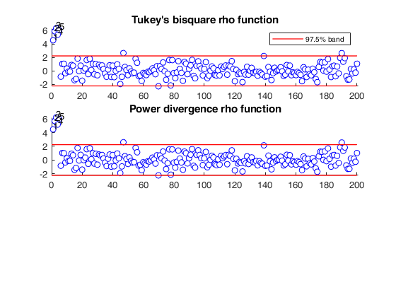
    If plots = 1, generates a plot with the robust residuals against index number. The confidence level used to draw the confidence bands for the residuals is given by the input option conflev. If conflev is not specified a nominal 0.975 confidence interval will be used.

    Example: 'plots',0

    Data Types: single | double

    yxsave —Save matrices X and y.scalar.

    If yxsave is equal to 1 the response vector y and data matrix X are saved into the output structure out.

    Default is 0, i.e. no saving is done.

    Example: 'yxsave',1

    Data Types: double

    Output Arguments

    expand all

    out — description Structure

    A structure containing the following fields

    Value Description
    beta

    vector containing the Tau estimator of regression coefficients

    scale

    scalar containing the estimate of the tau scale (sigma). This is the value of the objective function tau_scale = s_scale * average (\rho_2 (scaled residuals))

    bs

    p x 1 vector containing the units forming best subset associated with tau estimate of regression coefficient.

    residuals

    n x 1 vector containing the estimates of the robust scaled residuals

    outliers

    this output is present only if conflev has been specified. It is a vector containing the list of the units declared as outliers using confidence level specified in input scalar conflev

    conflev

    confidence level which is used to declare outliers.

    Remark: scalar out.conflev will be used to draw the horizontal line (confidence band) in the plot.

    singsub

    Number of subsets wihtout full rank. Notice that out.singsub > 0.1*(number of subsamples) produces a warning

    weights

    n x 1 vector containing the estimates of the weights

    rhofunc

    string identifying the rho function which has been used

    rhofuncparam

    vector which contains the additional parameters for the specified rho function which have been used. For hyperbolic rho function the value of k =sup CVC. For Hampel rho function the parameters a, b and c. This field is present only if input argument 'rhofunc' is 'hyperbolic' or 'hampel'.

    y

    Response vector y. The field is present only if option yxsave is set to 1.

    X

    Data matrix X. The field is present only if option yxsave is set to 1.

    class

    'Taureg'

    References

    Maronna, R.A., Martin D. and Yohai V.J. (2006), "Robust Statistics, Theory and Methods", Wiley, New York.

    Salibian-Barrera, M., Willems, G. and Zamar, R.H. (2008), The fast-tau estimator for regression, "Journal of Computational and Graphical Statistics", Vol. 17, pp. 659-682. [Referred below as SBWZ08].

    Yohai V.J. and Zamar R.H. (1988), High Breakdown-Point Estimates of Regression by Means of the Minimization of an Efficient Scale, "Journal of the American Statistical Association", Vol. 83, pp. 406-413.

    [Referred below as YZ88].

    Acknowledgements

    The kernel of the function is based on a MATLAB code downloaded from the web page of Dr. Matias Saliban-Barrera. However, all routines and subroutines have been completely redesigned, with considerable increase of the computational performance. Moreover in this function there is the possibility of choosing the rho (psi) function.

    See Also

    |

    This page has been automatically generated by our routine publishFS