Processing math: 0%

corrNominal

corrNominal measures strength of association between two unordered (nominal) categorical variables.

Syntax

Description

corrNominal computes , \Phi, Cramer's V, Goodman-Kruskal's \lambda_{y|x}, Goodman-Kruskal's \tau_{y|x}, and Theil's H_{y|x} (uncertainty coefficient).

All these indexes measure the association among two unordered qualitative variables.

If the input table is 2-by-2 indexes theta (cross product ratio), Q=(theta-1)/(theta+1) and U=Q=(sqrt(theta)-1)/(sqrt(theta)+1) are also computed Additional details about these indexes can be found in the "More About" section or in the "Output section" of this document.

example

out =corrNominal(N) corrNominal with all the default options.

example

out =corrNominal(N, Name, Value) Example of option conflev.

Examples

expand all

  • corrNominal with all the default options.
  • Rows of N indicate type of Bachelor degree: 'Economics' 'Law' 'Literature' Columns of N indicate employment type: 'Private_firm' 'Public_firm' 'Freelance' 'Unemployed'

    N=[150  80  20  50
    80  250  30  140
    30  50  0  120];
    out=corrNominal(N);
    Chi2 index
      221.2405
    
    pvalue Chi2 index
       5.6588e-45
    
    Phi index
        0.4704
    
    Cramer's V 
        0.3326
    
    Test of H_0: independence between rows and columns
                       Coeff         se       zscore       pval   
                      ________    ________    ______    __________
    
        CramerV         0.3326    0.024431    13.614             0
        GKlambdayx     0.22581    0.028383    7.9556    1.7764e-15
        tauyx         0.091674    0.013524    6.7788    1.2121e-11
        Hyx            0.08716    0.011265    7.7374    1.0214e-14
    
    -----------------------------------------
    Indexes and 95% confidence limits
                       Value      StandardError    ConflimL    ConflimU
                      ________    _____________    ________    ________
    
        CramerV         0.3326      0.024431        0.28471    0.37287 
        GKlambdayx     0.22581      0.028383        0.17018    0.28144 
        tauyx         0.091674      0.013524       0.065168    0.11818 
        Hyx            0.08716      0.011265       0.065082    0.10924 


  • Example of option conflev.
  • Use data from Goodman Kruskal (1954).

    N=[1768   807    189 47
    946 1387 746 53
    115 438 288 16];
    out=corrNominal(N,'conflev',0.99);
    Chi2 index
       1.0735e+03
    
    pvalue Chi2 index
      1.1244e-228
    
    Phi index
        0.3973
    
    Cramer's V 
        0.2810
    
    Test of H_0: independence between rows and columns
                       Coeff         se        zscore    pval
                      ________    _________    ______    ____
    
        CramerV        0.28095    0.0088396    31.784     0  
        GKlambdayx     0.19239     0.012158    15.825     0  
        tauyx         0.080883    0.0046282    17.476     0  
        Hyx           0.075341    0.0041619    18.102     0  
    
    -----------------------------------------
    Indexes and 99% confidence limits
                       Value      StandardError    ConflimL    ConflimU
                      ________    _____________    ________    ________
    
        CramerV        0.28095      0.0088396       0.25818     0.30241
        GKlambdayx     0.19239       0.012158       0.16108     0.22371
        tauyx         0.080883      0.0046282      0.068962    0.092805
        Hyx           0.075341      0.0041619      0.064621    0.086061


    Related Examples

    expand all

  • corrNominal with option dispresults.
  • N=[ 6 14 17 9;
    30 32 17 3];
    out=corrNominal(N,'dispresults',false);

  • Example which starts from the original data matrix.
  • N=[26 26 23 18 9;
    6 7 9 14 23];
    % From the contingency table reconstruct the original data matrix.
    n11=N(1,1); n12=N(1,2); n13=N(1,3); n14=N(1,4); n15=N(1,5);
    n21=N(2,1); n22=N(2,2); n23=N(2,3); n24=N(2,4); n25=N(2,5);
    x11=[1*ones(n11,1) 1*ones(n11,1)];
    x12=[1*ones(n12,1) 2*ones(n12,1)];
    x13=[1*ones(n13,1) 3*ones(n13,1)];
    x14=[1*ones(n14,1) 4*ones(n14,1)];
    x15=[1*ones(n15,1) 5*ones(n15,1)];
    x21=[2*ones(n21,1) 1*ones(n21,1)];
    x22=[2*ones(n22,1) 2*ones(n22,1)];
    x23=[2*ones(n23,1) 3*ones(n23,1)];
    x24=[2*ones(n24,1) 4*ones(n24,1)];
    x25=[2*ones(n25,1) 5*ones(n25,1)];
    % X original data matrix (in this case an array)
    X=[x11; x12; x13; x14; x15; x21; x22; x23; x24; x25];
    out=corrNominal(X,'datamatrix',true);

  • Example of option datamatrix combined with X defined as table.
  • Initial contingency matrix (2D array).

    N=[75   126
    76 203
    40 129
    36 125
    24 110
    41 222
    19 141];
    % Labels of the contingency matrix
    Party={'ACTIVIST DEMOCRATIC', 'DEMOCRATIC', ...
    'SIMPATIZING DEMOCRATIC', 'INDEPENDENT', ...
    'LIKING REPUBLICAN', 'REPUBLICAN', ...
    'ACTIVIST REPUBLICAN'};
    DeathPenalty={'AGAINST' 'FAVORABLE'};
    Ntable=array2table(N,'RowNames',Party,'VariableNames',DeathPenalty);
    % From the contingency table reconstruct the original data matrix now
    % using FSDA function
    % The output is a cell arrary
    Xcell=crosstab2datamatrix(Ntable);
    Xtable=cell2table(Xcell);
    % call function corrNominal using first argument as input data matrix
    % in table format and option datamatrix set to true
    out=corrNominal(Xtable,'datamatrix',true);

  • Example: compare confidence interval for Cramer V.
  • Use the 4 possible methods

    method={'ncchisq', 'ncchisqadj', 'fisher' 'fisheradj'};
    % Use a contingency table referred to type of job vs wine delivery
    rownam={'Butcher' 'Carpenter' 'Carter' 'Farmer' 'Hunter' 'Miller' 'Taylor'};
    colnam={'Wine not delivered' 'Wine delivered'};
    N=[85 9
    214 56
    212 19
    100 17
    139 15
    109 16
    172 29];
    Ntable=array2table(N,'RowNames',rownam,'VariableNames',colnam);
    ConfintV=zeros(4,2);
    for i=1:4
    out=corrNominal(Ntable,'conflimMethodCramerV',method{i});
    ConfintV(i,:)=out.ConfLimtable{'CramerV',3:4};
    end
    disp(array2table(ConfintV,'RowNames',method,'VariableNames',{'Lower' 'Upper'}))
    Chi2 index
       21.0290
    
    pvalue Chi2 index
        0.0018
    
    Phi index
        0.1328
    
    Cramer's V 
        0.1328
    
    Test of H_0: independence between rows and columns
                       Coeff         se        zscore      pval   
                      ________    _________    ______    _________
    
        CramerV        0.13282      0.04149    3.2013    0.0013679
        GKlambdayx           0            0       NaN          NaN
        tauyx         0.017642    0.0078826    2.2381     0.025218
        Hyx           0.021875    0.0095422    2.2924     0.021883
    
    -----------------------------------------
    Indexes and 95% confidence limits
                       Value      StandardError    ConflimL     ConflimU
                      ________    _____________    _________    ________
    
        CramerV        0.13282        0.04149       0.051504     0.17582
        GKlambdayx           0              0              0           0
        tauyx         0.017642      0.0078826      0.0021921    0.033091
        Hyx           0.021875      0.0095422      0.0031721    0.040577
    
    Chi2 index
       21.0290
    
    pvalue Chi2 index
        0.0018
    
    Phi index
        0.1328
    
    Cramer's V 
        0.1328
    
    Test of H_0: independence between rows and columns
                       Coeff         se        zscore       pval   
                      ________    _________    ______    __________
    
        CramerV        0.13282     0.023037    5.7657    8.1331e-09
        GKlambdayx           0            0       NaN           NaN
        tauyx         0.017642    0.0078826    2.2381      0.025218
        Hyx           0.021875    0.0095422    2.2924      0.021883
    
    -----------------------------------------
    Indexes and 95% confidence limits
                       Value      StandardError    ConflimL     ConflimU
                      ________    _____________    _________    ________
    
        CramerV        0.13282       0.023037       0.087671     0.18959
        GKlambdayx           0              0              0           0
        tauyx         0.017642      0.0078826      0.0021921    0.033091
        Hyx           0.021875      0.0095422      0.0031721    0.040577
    
    Chi2 index
       21.0290
    
    pvalue Chi2 index
        0.0018
    
    Phi index
        0.1328
    
    Cramer's V 
        0.1328
    
    Test of H_0: independence between rows and columns
                       Coeff         se        zscore      pval   
                      ________    _________    ______    _________
    
        CramerV        0.13282     0.028675     4.632    3.621e-06
        GKlambdayx           0            0       NaN          NaN
        tauyx         0.017642    0.0078826    2.2381     0.025218
        Hyx           0.021875    0.0095422    2.2924     0.021883
    
    -----------------------------------------
    Indexes and 95% confidence limits
                       Value      StandardError    ConflimL     ConflimU
                      ________    _____________    _________    ________
    
        CramerV        0.13282       0.028675       0.076621     0.18818
        GKlambdayx           0              0              0           0
        tauyx         0.017642      0.0078826      0.0021921    0.033091
        Hyx           0.021875      0.0095422      0.0031721    0.040577
    
    Chi2 index
       21.0290
    
    pvalue Chi2 index
        0.0018
    
    Phi index
        0.1328
    
    Cramer's V 
        0.1328
    
    Test of H_0: independence between rows and columns
                       Coeff         se        zscore       pval   
                      ________    _________    ______    __________
    
        CramerV        0.13282     0.028646    4.6366    3.5418e-06
        GKlambdayx           0            0       NaN           NaN
        tauyx         0.017642    0.0078826    2.2381      0.025218
        Hyx           0.021875    0.0095422    2.2924      0.021883
    
    -----------------------------------------
    Indexes and 95% confidence limits
                       Value      StandardError    ConflimL     ConflimU
                      ________    _____________    _________    ________
    
        CramerV        0.13282       0.028646       0.076676     0.18824
        GKlambdayx           0              0              0           0
        tauyx         0.017642      0.0078826      0.0021921    0.033091
        Hyx           0.021875      0.0095422      0.0031721    0.040577
    
                       Lower       Upper 
                      ________    _______
    
        ncchisq       0.051504    0.17582
        ncchisqadj    0.087671    0.18959
        fisher        0.076621    0.18818
        fisheradj     0.076676    0.18824


  • CorrNominal when input is 2 by 2.
  • Indexes theta=cross product ratio, Q and U are also computed.

    % X=advertisment memory (rows)
    % Y=product purchase (columns)
    N= [87 188;
    42 406];
    nam=["Yes" "No"];
    Ntable=array2table(N,"RowNames",nam,"VariableNames",nam);
    disp('Input 2x2 contingency table')
    table(Ntable,RowNames=["X=advertisment memory" "advertisment memory "],VariableNames="Y=Product purchase")
    out=corrNominal(Ntable)
    Input 2x2 contingency table
    
    ans =
    
      2×1 table
    
                                 Y=Product purchase
                                 __________________
    
                                        Yes    No  
                                        ___    ___ 
                                                   
        X=advertisment memory    Yes    87     188 
        advertisment memory      No     42     406 
    
    Chi2 index
       57.6071
    
    pvalue Chi2 index
       3.2006e-14
    
    Phi index
        0.2823
    
    Cramer's V 
        0.2823
    
    -------------------------------
    2x2 contingency table indexes
    th=cross product ratio
        4.4734
    
    Cross product ratio in the interval [-1 1]. Index Q=(th-1)/(th+1)
        0.6346
    
    Cross product ratio in the interval [-1 1]. Index U=(sqrt(th)-1)/(sqrt(th)+1)
        0.3580
    
    -------------------------------
    Test of H_0: independence between rows and columns
                       Coeff         se       zscore       pval   
                      ________    ________    ______    __________
    
        CramerV        0.28227    0.037189    7.5902    3.1974e-14
        GKlambdayx           0           0       NaN           NaN
        tauyx         0.079678    0.020787    3.8331    0.00012653
        Hyx           0.082782    0.021327    3.8816    0.00010376
    
    -----------------------------------------
    Indexes and 95% confidence limits
                       Value      StandardError    ConflimL    ConflimU
                      ________    _____________    ________    ________
    
        CramerV        0.28227      0.037189        0.20938    0.35516 
        GKlambdayx           0             0              0          0 
        tauyx         0.079678      0.020787       0.038937    0.12042 
        Hyx           0.082782      0.021327       0.040983    0.12458 
    
    
    out = 
    
      struct with fields:
    
                         N: [2×2 double]
                    Ntable: [2×2 table]
                      Chi2: 57.6071
                  Chi2pval: 3.2006e-14
                       Phi: 0.2823
                   CramerV: [0.2823 0.0372 7.5902 3.1974e-14]
                GKlambdayx: [0 0 NaN NaN]
                     tauyx: [0.0797 0.0208 3.8331 1.2653e-04]
                       Hyx: [0.0828 0.0213 3.8816 1.0376e-04]
                   ConfLim: [4×4 double]
              ConfLimtable: [4×4 table]
                   TestInd: [4×4 double]
              TestIndtable: [4×4 table]
                     theta: 4.4734
                         Q: 0.6346
                         U: 0.3580
              Contrib2Chi2: [2×2 double]
         Contrib2Chi2table: [2×2 table]
               Contrib2Hyx: [2×2 double]
          Contrib2Hyxtable: [2×2 table]
             Contrib2tauyx: [2×2 double]
        Contrib2tauyxtable: [2×2 table]


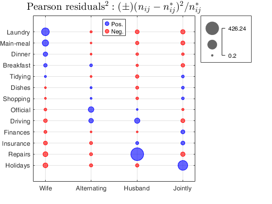
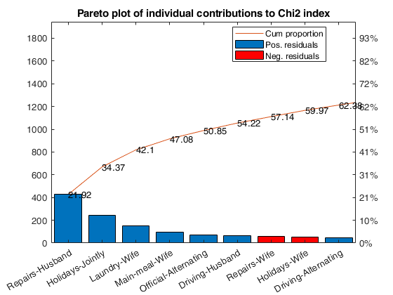
  • Example of call to CorrNominal with optional input argument plots.
  • Load the Housetasks data (a contingency table containing the frequency of execution of 13 house tasks in the couple).

    N=[156  14  2  4;
    124  20  5  4;
    77  11  7  13;
    82  36  15  7;
    53  11  1  57;
    32  24  4  53;
    33  23  9  55;
    12  46  23  15;
    10  51  75  3;
    13  13  21  66;
    8  1  53  77;
    0  3  160  2;
    0  1  6  153];
    rowslab={'Laundry' 'Main-meal' 'Dinner' 'Breakfast' 'Tidying' 'Dishes' ...
    'Shopping' 'Official' 'Driving' 'Finances' 'Insurance'...
    'Repairs' 'Holidays'};
    colslab={'Wife'  'Alternating'  'Husband'  'Jointly'};
    Ntable=array2table(N,'VariableNames',colslab,'RowNames',rowslab);
    % Call to corrNominal with option 'plots',true
    corrNominal(Ntable,'plots',true);
    Chi2 index
       1.9445e+03
    
    pvalue Chi2 index
         0
    
    Phi index
        1.0559
    
    Cramer's V 
        0.6096
    
    Test of H_0: independence between rows and columns
                       Coeff        se       zscore    pval
                      _______    ________    ______    ____
    
        CramerV       0.60963    0.016701    36.502     0  
        GKlambdayx    0.50787    0.018427    27.561     0  
        tauyx         0.40671    0.013787      29.5     0  
        Hyx           0.40833    0.013767    29.659     0  
    
    -----------------------------------------
    Indexes and 95% confidence limits
                       Value     StandardError    ConflimL    ConflimU
                      _______    _____________    ________    ________
    
        CramerV       0.60963      0.016701       0.57689     0.63133 
        GKlambdayx    0.50787      0.018427       0.47175     0.54398 
        tauyx         0.40671      0.013787       0.37969     0.43374 
        Hyx           0.40833      0.013767       0.38134     0.43531 
    
    
    Click here for the graphical output of this example (link to Ro.S.A. website)

    Input Arguments

    expand all

    N — Contingency table (default) or n-by-2 input dataset. Matrix or Table.

    Matrix or table which contains the input contingency table (say of size I-by-J) or the original data matrix.

    In this last case N=crosstab(N(:,1),N(:,2)). As default procedure assumes that the input is a contingency table.

    If N is a data matrix (supplied as a a n-by-2 cell array of strings, or n-by-2 array or n-by-2 table) optional input datamatrix must be set to true.

    Data Types: single| double

    Name-Value Pair Arguments

    Specify optional comma-separated pairs of Name,Value arguments. Name is the argument name and Value is the corresponding value. Name must appear inside single quotes (' '). You can specify several name and value pair arguments in any order as Name1,Value1,...,NameN,ValueN.

    Example: 'conflev',0.99 , 'conflimMethodCramerV','fisheradj' , 'dispresults',false , 'Lr',{'a' 'b' 'c'} , 'Lc',{'c1' c2' 'c3' 'c4'} , 'datamatrix',true , 'NoStandardErrors',true , 'plots',true

    conflev —Confidence levels to be used to compute confidence intervals.scalar.

    The default value of conflev is 0.95, that is 95 per cent confidence intervals are computed for all the indexes (note that this option is ignored if NoStandardErrors=true).

    Example: 'conflev',0.99

    Data Types: double

    conflimMethodCramerV —method to compute confidence interval for CramerV.character.

    Character which identifies the method to use to compute the confidence interval for Cramer index. Default value is 'ncchisq'. Possible values are 'ncchisq', 'ncchisqadj', 'fisher' or 'fisheradj'; 'ncchisq' uses the non central chi2. 'ncchisq' uses the non central chi2 adjusted for the degrees of fredom. 'fisher' uses the Fisher z-transformation and 'fisheradj' uses the fisher z-transformation and bias correction.

    Example: 'conflimMethodCramerV','fisheradj'

    Data Types: character

    dispresults —Display results on the screen.boolean.

    If dispresults is true (default) it is possible to see on the screen all the summary results of the analysis.

    Example: 'dispresults',false

    Data Types: Boolean

    Lr —Vector of row labels.cell.

    Cell containing the labels of the rows of the input contingency matrix N. This option is unnecessary if N is a table, because in this case Lr=N.Properties.RowNames;

    Example: 'Lr',{'a' 'b' 'c'}

    Data Types: cell array of strings

    Lc —Vector of column labels.cell.

    Cell containing the labels of the columns of the input contingency matrix N. This option is unnecessary if N is a table, because in this case Lc=N.Properties.VariableNames;

    Example: 'Lc',{'c1' c2' 'c3' 'c4'}

    Data Types: cell array of strings

    datamatrix —Data matrix or contingency table.boolean.

    If datamatrix is true the first input argument N is forced to be interpreted as a data matrix, else if the input argument is false N is treated as a contingency table. The default value of datamatrix is false, that is the procedure automatically considers N as a contingency table. In case datamatrix is true N can be a cell of size n-by-2 containing the two grouping variables or a numeric array of size n-by-2 or a table of size n-by-2.

    Example: 'datamatrix',true

    Data Types: logical

    NoStandardErrors —Just indexes without standard errors and p-values.boolean.

    if NoStandardErrors is true just the indexes are computed without standard errors and p-values. That is no inferential measure is given. The default value of NoStandardErrors is false.

    Example: 'NoStandardErrors',true

    Data Types: Boolean

    plots —balloonplot of squared Pearson residuals and Pareto plot of squared Pearson residuals.boolean.

    If plots is true the following two plots of Pearson squared residuals are shown on the screen.

    1) a bubble plot (ballonplot);

    2) a Pareto plot.

    In both plots entries of the contingency table associated with positive association (positive residuals) are shown in blue while those associated with negative association (negative residuals) are shown in red.

    The default value of plots is false.

    Example: 'plots',true

    Data Types: Boolean

    Output Arguments

    expand all

    out — description Structure

    Structure which contains the following fields:

    Value Description
    N

    I-by-J-array containing contingency table referred to active rows (i.e. referred to the rows which participated to the fit).

    The (i,j)-th element is equal to n_{ij}, i=1, 2, \ldots, I and j=1, 2, \ldots, J. The sum of the elements of out.N is n (the grand total).

    Ntable

    same as out.N but in table format (with row and column names).

    This output is present just if your MATLAB version is not<2013b.

    Chi2

    scalar containing \chi^2 index.

    Chi2pval

    scalar containing pvalue of the \chi^2 index.

    Phi

    \Phi index. Phi is a chi-square-based measure of association that involves dividing the chi-square statistic by the sample size and taking the square root of the result. More precisely \Phi= \sqrt{ \frac{\chi^2}{n} } This index lies in the interval [0 , \sqrt{\min[(I-1),(J-1)]}.

    CramerV

    1 x 4 vector which contains Cramer's V index, standard error, z test, and p-value. Cramer'V index is index \Phi divided by its maximum. More precisely V= \sqrt{\frac{\Phi}{\min[(I-1),(J-1)]}}=\sqrt{\frac{\chi^2}{n \min[(I-1),(J-1)]}}

    The range of Cramer index is [0, 1]. A Cramer's V in the range of [0, 0.3] is considered as weak, [0.3,0.7] as medium and > 0.7 as strong.

    The way in which the confidence interval for this index is specified in input option conflimMethodCramerV.

    If conflimMethodCramerV is 'ncchisq', 'ncchisqadj' we first find a confidence interval for the non centrality parameter \Delta of the \chi^2 distribution with df=(I-1)(J-1) degrees of freedom. (see Smithson (2003); pp. 39-41) [\Delta_L \Delta_U]. If input option conflimMethodCramerV is 'ncchisq', confidence interval for \Delta is transformed into one for V by the following transformation

    V_L=\sqrt{\frac{\Delta_L }{n \min[(I-1),(J-1)]}} and V_U=\sqrt{\frac{\Delta_U }{n \min[(I-1),(J-1)]}} If input option conflimMethodCramerV is 'ncchisqadj', confidence interval for \Delta is transformed into one for V by the following transformation V_L=\sqrt{\frac{\Delta_L+ df }{n \min[(I-1),(J-1)]}} and V_U=\sqrt{\frac{\Delta_U+ df }{n \min[(I-1),(J-1)]}}

    GKlambdayx

    1 x 4 vector which contains index \lambda_{y|x} of Goodman and Kruskal standard error, z test, and p-value.

    \lambda_{y|x} = \sum_{i=1}^I \frac{r_i- r}{n-r} r_i =\max(n_{ij}) r =\max(n_{.j})

    tauyx

    1 x 4 vector which contains tau index \tau_{y|x}, standard error, ztest and p-value.

    \tau_{y|x}= \frac{\sum_{i=1}^I \sum_{j=1}^J f_{ij}^2/f_{i.} -\sum_{j=1}^J f_{.j}^2 }{1-\sum_{j=1}^J f_{.j}^2 }

    Hyx

    1 x 4 vector which contains the uncertainty coefficient index (proposed by Theil) H_{y|x}, standard error, ztest and p-value.

    H_{y|x}= \frac{\sum_{i=1}^I \sum_{j=1}^J f_{ij} \log( f_{ij}/ (f_{i.}f_{.j}))}{\sum_{j=1}^J f_{.j} \log f_{.j} }

    TestInd

    4-by-4 array containing index values (first column), standard errors (second column), zscores (third column), p-values (fourth column).

    TestIndtable

    4-by-4 table containing index values (first column), standard errors (second column), zscores (third column), p-values (fourth column).

    ConfLim

    4-by-4 array containing index values (first column), standard errors (second column), lower confidence limit (third column), upper confidence limit (fourth column).

    ConfLimtable

    4-by-4 table containing index values (first column), standard errors (second column), lower confidence limit (third column), upper confidence limit (fourth column).

    theta

    cross product ratio. This index is computed just if the input table is 2-by-2

    Q

    cross product ratio in the interval [-1 1] using the Q rescaling Q=(th-1)/(th+1). This index is computed just if the input table is 2-by-2

    U

    cross product ratio in the interval [-1 1] using the U rescaling U=(sqrt(th)-1)/(sqrt(th)+1). This index is computed just if the input table is 2-by-2

    Contrib2Chi2

    I x J array containing the contributions (with sign) to the Chi2 index.

    Note that sum(abs(out.Contrib2chi),'all')=out.Chi2.

    Contrib2Chi2table

    same of out.Contrib2chi but in table format

    Contrib2Hyx

    I x J array containing the contributions to the Hyx index.

    Note that sum(out.Contrib2Hyx,'all')=out.Hyx.

    Contrib2Hyxtable

    same of out.Contrib2Hyx but in table format

    Contrib2tauyx

    I x J array containing the contributions to the tauyx index.

    Note that sum(out.Contrib2tauyx,'all')=out.tauyx.

    Contrib2tauyxtable

    same of out.Contrib2tauyx but in table format

    More About

    expand all

    Additional Details

    In the contingency table N of size I \times J, whose i,j entry is n_{ij}, the Pearson residuals are defined as \frac{n_{ij}-n_{ij}^*}{\sqrt{n_{ij}^*}} where n_{ij}^* is the theoretical frequency under the independence hypothesis. The sum of the squares of the Pearson residuals is equal to the \chi^2 statistic to test the independence between rows and columns of the contingency table.

    \lambda_{y|x} is a measure of association that reflects the proportional reduction in error when values of the independent variable (variable in the rows of the contingency table) are used to predict values of the dependent variable (variable in the columns of the contingency table). The range of \lambda_{y|x} is [0, 1]. A value of 1 means that the independent variable perfectly predicts the dependent variable. On the other hand, a value of 0 means that the independent variable does not help in predicting the dependent variable.

    More generally, let V(y) a measure of variation for the marginal distribution (f_{.1}=n_{.1}/n, ..., f_{.J}=n_{.J}/n) of the response y and let V(y|i) denote the same measure computed for the conditional distribution (f_{1|i}=n_{1|i}/n, ..., f_{J|i}=n_{J|i}/n) of y at the i-th setting of the explanatory variable x. A proportional reduction in variation measure has the form.

    \frac{V(y) - E[V(y|x)]}{V(y|x)} where E[V(y|x)] is the expectation of the conditional variation taken with respect to the distribution of x. When x is a categorical variable having marginal distribution, (f_{1.}, \ldots, f_{I.}), E[V(y|x)]= \sum_{i=1}^I (n_{i.}/n) V(y|i) = \sum_{i=1}^I f_{i.} V(y|i) If we take as measure of variation V(y) the Gini coefficient V(y)=1 -\sum_{j=1}^J f_{.j} \qquad V(y|i)=1 -\sum_{j=1}^J f_{j|i}

    we obtain the index of proportional reduction in variation \tau_{y|x} of Goodman and Kruskal.

    \tau_{y|x}= \frac{\sum_{i=1}^I \sum_{j=1}^J f_{ij}^2/f_{i.} -\sum_{j=1}^J f_{.j}^2 }{1-\sum_{j=1}^J f_{.j}^2 } If, on the other hand, we take as measure of variation V(y) the entropy index V(y)=-\sum_{j=1}^J f_{.j} \log f_{.j} \qquad V(y|i) -\sum_{j=1}^J f_{j|i} \log f_{j|i}

    we obtain the index H_{y|x}, (uncertainty coefficient of Theil).

    H_{y|x}= \frac{\sum_{i=1}^I \sum_{j=1}^J f_{ij} \log( f_{ij}/ (f_{i.}f_{.j}))}{\sum_{j=1}^J f_{.j} \log f_{.j} }

    The range of \tau_{y|x} and H_{y|x} is [0 1].

    A large value of of the index represents a strong association, in the sense that we can guess y much better when we know x than when we do not.

    In other words, \tau_{y|x}=H_{y|x} =1 is equivalent to no conditional variation in the sense that for each i, n_{j|i}=1. For example, a value of: \tau_{y|x}=0.85 indicates that knowledge of x reduces error in predicting values of y by 85 per cent (when the variation measure which is used is the Gini's index).

    H_{y|x}=0.85 indicates that knowledge of x reduces error in predicting values of y by 85 per cent (when variation measure which is used is the entropy index) Remark: if the contingency table is of size 2x2 the following indexes are also computed theta=cross product ratio, index Q

    Q= \frac{\theta-1}{\theta+1} and U U= \frac{\sqrt{\theta}-1}{\sqrt{\theta}+1}

    References

    Agresti, A. (2002), "Categorical Data Analysis", John Wiley & Sons. [pp.

    23-26]

    Goodman, L.A. and Kruskal, W.H. (1959), Measures of association for cross classifications II: Further Discussion and References, "Journal of the American Statistical Association", Vol. 54, pp. 123-163.

    Goodman, L.A. and Kruskal, W.H. (1963), Measures of association for cross classifications III: Approximate Sampling Theory, "Journal of the American Statistical Association", Vol. 58, pp. 310-364.

    Goodman, L.A. and Kruskal, W.H. (1972), Measures of association for cross classifications IV: Simplification of Asymptotic Variances, "Journal of the American Statistical Association", Vol. 67, pp. 415-421.

    Liebetrau, A.M. (1983), "Measures of Association", Sage University Papers Series on Quantitative Applications in the Social Sciences, 07-004, Newbury Park, CA: Sage. [pp. 49-56]

    Smithson, M.J. (2003), "Confidence Intervals", Quantitative Applications in the Social Sciences Series, No. 140. Thousand Oaks, CA: Sage. [pp.

    39-41]

    Acknowledgements

    This page has been automatically generated by our routine publishFS