
|
corrNominal |
corrpdf |
 |
corrOrdinal
corrOrdinal measures strength of association between two ordered categorical variables.
Description
corrOrdinal computes Goodman-Kruskal's , \tau_a, \tau_b, \tau_c of Kendall and d_{y|x} of Somers.
All these indexes measure the correlation among two ordered qualitative variables and go between -1 and 1. The sign of the coefficient indicates the direction of the relationship, and its absolute value indicates the strength, with larger absolute values indicating stronger relationships. Values close to an absolute value of 1 indicate a strong relationship between the two variables. Values close to 0 indicate little or no relationship. More in detail: \gamma is a symmetric measure of association.
Kendall's \tau_a is a symmetric measure of association that does not take ties into account. Ties happen when both members of the data pair have the same value.
Kendall's \tau_b is a symmetric measure of association which takes ties into account. Even if \tau_b ranges from -1 to 1, a value of -1 or +1 can be obtained only from square tables.
\tau_c (also called Stuart-Kendall \tau_c) is a symmetric measure of association which makes an adjustment for table size in addition to a correction for ties. Even if \tau_c ranges from -1 to 1, a value of -1 or +1 can be obtained only from square tables.
Somers' d is an asymmetric extension of \tau_b in that it uses a correction only for pairs that are tied on the independent variable (which in this implementation it is assumed to be on the rows of the contingency table).
Additional details about these indexes can be found in the "More About" section of this document.
Compare calculation of tau-b with that which comes from
Matlab function corr.out
=corrOrdinal(N,
Name, Value)
Examples
 corrOrdinal with all the default options.
corrOrdinal with all the default options.Rows of N indicate the results of a written test with levels: 'Sufficient' 'Good' Very good' Columns of N indicate the results of an oral test with levels: 'Sufficient' 'Good' Very good'
N=[20    40    20;
10    45    45;
0     5    15];
out=corrOrdinal(N);
% Because the asymptotic 95 per cent confidence limits do not contain
% zero, this indicates a strong positive association between the
% written and the oral examination.
Test of H_0: independence between rows and columns
The standard errors are computed under H_0
              Coeff        se       zscore       pval
             _______    ________    ______    __________

    gamma        0.5    0.098239    5.0896     3.588e-07
    taua     0.18342    0.047553    3.8571    0.00011474
    taub     0.30557    0.060038    5.0896     3.588e-07
    tauc     0.27375    0.053786    5.0896     3.588e-07
    dyx      0.31466    0.061823    5.0896     3.588e-07

-----------------------------------------
Indexes and 95% confidence limits
The standard error are computed under H_1
              Value     StandardError    ConflimL    ConflimU
             _______    _____________    ________    ________

    gamma        0.5        0.0876       0.32831     0.67169
    taua     0.18342      0.011904       0.16009     0.20675
    taub     0.30557       0.05852       0.19087     0.42027
    tauc     0.27375      0.053786       0.16833     0.37917
    dyx      0.31466      0.059899       0.19726     0.43205
Compare calculation of tau-b with that which comes from
Matlab function corr.
Compare calculation of tau-b with that which comes from
Matlab function corr.
% Starting from a contingency table, create the original data matrix to
% te able to call corr.
N=[20    23    20;
21    25    22;
18     18    19];
n11=N(1,1); n12=N(1,2); n13=N(1,3);
n21=N(2,1); n22=N(2,2); n23=N(2,3);
n31=N(3,1); n32=N(3,2); n33=N(3,3);
x11=[1*ones(n11,1) 1*ones(n11,1)];
x12=[1*ones(n12,1) 2*ones(n12,1)];
x13=[1*ones(n13,1) 3*ones(n13,1)];
x21=[2*ones(n21,1) 1*ones(n21,1)];
x22=[2*ones(n22,1) 2*ones(n22,1)];
x23=[2*ones(n23,1) 3*ones(n23,1)];
x31=[3*ones(n31,1) 1*ones(n31,1)];
x32=[3*ones(n32,1) 2*ones(n32,1)];
x33=[3*ones(n33,1) 3*ones(n33,1)];
% X original data matrix
X=[x11; x12; x13; x21; x22; x23; x31; x32; x33];
% Find taub and pvalue of taub using MATLAB routine corr
[RHO,pval]=corr(X,'type','Kendall');
% Compute tau-b using FSDA corrOrdinal routine.
out=corrOrdinal(X,'datamatrix',true,'dispresults',false);
disp(['tau-b from MATLAB routine corr=' num2str(RHO(1,2))])
disp(['tau-b from FSDA routine corrOrdinal=' num2str(out.taub(1))])
% Remark the p-values are slightly different
disp(['pvalue of H0:taub=0 from MATLAB routine corr=' num2str(pval(1,2))])
disp(['pvalue of H0:taub=0 from FSDA routine corrOrdinal=' num2str(out.taub(4))])
tau-b from MATLAB routine corr=0.0083449
tau-b from FSDA routine corrOrdinal=0.0083449
pvalue of H0:taub=0 from MATLAB routine corr=0.89952
pvalue of H0:taub=0 from FSDA routine corrOrdinal=0.89914
Related Examples
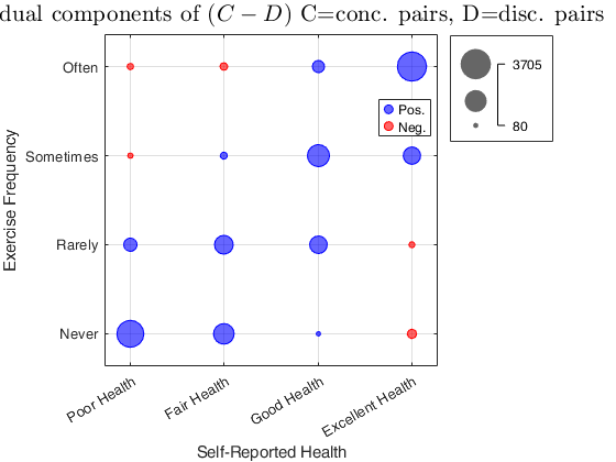
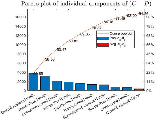
Example 1 of use of option plots.
Example 1 of use of option plots.Exercise Frequency vs. Self-Reported Health
load SportHealth.mat
out=corrOrdinal(SportHealth,'plots',true);
% It is clear the positive relationship between
% 'Self-Reported Health' and 'Exercise Frequency'
Test of H_0: independence between rows and columns
The standard errors are computed under H_0
              Coeff        se       zscore    pval
             _______    ________    ______    ____

    gamma    0.59385    0.053088    11.186     0
    taua     0.33958     0.03852    8.8157     0
    taub     0.45635    0.040796    11.186     0
    tauc     0.45128    0.040343    11.186     0
    dyx       0.4525    0.040451    11.186     0

-----------------------------------------
Indexes and 95% confidence limits
The standard error are computed under H_1
              Value     StandardError    ConflimL    ConflimU
             _______    _____________    ________    ________

    gamma    0.59385       0.04837       0.49905     0.68866
    taua     0.33958      0.011291       0.31745     0.36171
    taub     0.45635      0.040331        0.3773      0.5354
    tauc     0.45128      0.040343       0.37221     0.53036
    dyx       0.4525      0.040106       0.37389     0.53111
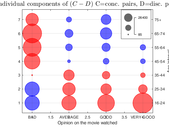
Example 2 of use of option plots.
Example 2 of use of option plots.Opinion on the movie watched and age interval
load cinema.mat
out=corrOrdinal(cinema,'plots',true);
% It is clear the negative relationship between
% age and satisfaction towards the watched movie
Test of H_0: independence between rows and columns
The standard errors are computed under H_0
              Coeff         se       zscore        pval
             ________    ________    _______    __________

    gamma    -0.22239    0.033693    -6.6004    4.0994e-11
    taua     -0.10884    0.018121    -6.0064    1.8967e-09
    taub     -0.15598    0.023632    -6.6004    4.0994e-11
    tauc     -0.14501     0.02197    -6.6004    4.0994e-11
    dyx      -0.12946    0.019614    -6.6004    4.0994e-11

-----------------------------------------
Indexes and 95% confidence limits
The standard error are computed under H_1
             Value    StandardError    ConflimL    ConflimU
             _____    _____________    ________    ________

    gamma      0         0.033312         0           0
    taua       0        0.0035492         0           0
    taub       0         0.023518         0           0
    tauc       0          0.02197         0           0
    dyx        0         0.019609         0           0

Input Arguments
Output Arguments
More About
References
Agresti, A. (2002), "Categorical Data Analysis", John Wiley & Sons. [pp.
57-59]
Agresti, A. (2010), "Analysis of Ordinal Categorical Data", Second Edition, Wiley, New York, pp. 194-195.
Goktas, A. and Oznur, I. (2011), A comparision of the most commonly used measures of association for doubly ordered square contingency tables via simulation, "Metodoloski zvezki", Vol. 8, pp. 17-37,
Goodman, L.A. and Kruskal, W.H. (1954), Measures of association for cross classifications, "Journal of the American Statistical Association", Vol. 49, pp. 732-764.
Goodman, L.A. and Kruskal, W.H. (1959), Measures of association for cross classifications II: Further Discussion and References, "Journal of the American Statistical Association", Vol. 54, pp. 123-163.
Goodman, L.A. and Kruskal, W.H. (1963), Measures of association for cross classifications III: Approximate Sampling Theory, "Journal of the American Statistical Association", Vol. 58, pp. 310-364.
Goodman, L.A. and Kruskal, W.H. (1972), Measures of association for cross classifications IV: Simplification of Asymptotic Variances, "Journal of the American Statistical Association", Vol. 67, pp. 415-421.
Hollander, M, Wolfe, D.A., Chicken, E. (2014), "Nonparametric Statistical Methods", Third edition, Wiley,
Liebetrau, A.M. (1983), "Measures of Association", Sage University Papers Series on Quantitative Applications in the Social Sciences, 07-004, Newbury Park, CA: Sage. [pp. 49-56]
SAS documentation (2009), See http://support.sas.com/documentation/cdl/en/statugfreq/63124/PDF/default/statugfreq.pdf, pp. 1738-1740.
Morton, B.B. and Benedetti, J.K. (1977), Sampling Behavior of Tests for Correlation in Two-Way Contingency Tables, "Journal of the American Statistical Association", Vol. 72, pp. 309-315.
Simon, G. (1978), Alternative analysis for the singly ordered contingency table, "Journal of the American Statistical Association", Vol. 69, pp. 971-976.
Acknowledgements
This file was inspired by Trujillo-Ortiz, A. and R. Hernandez-Walls.
gkgammatst: Goodman-Kruskal's gamma test. URL address http://www.mathworks.com/matlabcentral/fileexchange/42645-gkgammatst
See Also
crosstab
|
rcontFS
|
CressieRead
|
corr
|
corrNominal
|
|
corrNominal |
corrpdf |
|
|
|
Functions |
|
• The developers of the toolbox • The forward search group • Terms of Use • Acknowledgments