ctlcurvesplot

dempk

ctsub

ctsub computes numerical integration from x(1) to z(i) of y=f(x).

expand all in page

Syntax

a=ctsub(x,y,z)example
a=ctsub(x,y,z,Trapezoid)example

Description

For a function defined $y=f(x)$ with $n$ pairs $(x_1,y_1)$ $\ldots$ $(x_n,y_n)$ , with $x_1 \leq x_2 \leq, \ldots, \leq x_n$ this routine computes the (approximate) integral using the trapezoidal rule $a_i = \int_{x_1}^{z_i} f(x) dx$ For further details see the section More About.

example

a =ctsub(x, y, z) Transform a linear relation.

example

a =ctsub(x, y, z, Trapezoid) Comparison with MATLAB function cumtrapz.

Examples

expand all

Transform a linear relation.

n=1000;
x=sort(randn(n,1))+10;
y=1+2*x+ randn(n,1);
% y(50:70)=-5;
z=randn(n,1);
a=ctsub(x,y,z);
subplot(2,1,1)
plot(x,y)
subplot(2,1,2)
plot(x,a)

Comparison with MATLAB function cumtrapz.

n=1000;
x=sort(randn(n,1));
y=randn(n,1);
% If the third argument of ctsub is equal to the first
% argument then the output of cumtraps and ctsub is exactly the same.
res=cumtrapz(x,y);
res1=ctsub(x,y,x);
disp(max(abs(res-res1)))

Related Examples

expand all

Apply ctsub to heteroskedastic data.

n=1000;
x=10*sort(randn(n,1))+10;
% The variance of y depends on x.
y=1+1*x+ 10*x.*randn(n,1);
% Upper limits of integration.
z=rand(n,1)*100-50;
a=ctsub(x,y,z);
subplot(2,1,1)
plot(x,y)
title('Original data')
subplot(2,1,2)
plot(x,a)
title('Transformed data after the variance stabilizing transformation')

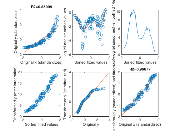
Example of application of routine ctsub inside AVAS.

Generate the data

rng(2000)
la=0;
n=100;
X=10*rand(n,1);
sigma=0.1;
a=2;
b=0.3;
y=a+b*X+sigma*randn(n,1);
% The correct transformation is log
y=normBoxCox(y,1,la,'inverse',true);
% Data standardization
y=zscore(y);
X=zscore(X);
out=fitlm(X,y);
yhat=out.Fitted;
res=y-yhat;
figure
nr=2;
nc=3;
subplot(nr,nc,1)
plot(X,y,'o')
hold('on')
[xsor,ordx]=sort(X);
yordx=yhat(ordx);
plot(xsor,yordx)
xlabel('Original x (standardized)')
ylabel('Original y (standardized)')
title(['R2=' num2str(out.Rsquared.Ordinary)])
subplot(nr,nc,2)
[yhatsor,ordyhat]=sort(yhat);
% Residuals sorted using the indexes of sorted fitted values
resordyhat=res(ordyhat);
yordyhat=y(ordyhat);
scatter(yhatsor,resordyhat)
xlabel('Sorted fitted values')
ylabel('Residuals (e) in correspondence of sorted fitted values')
% z2 = log abs value of the residuals
% ztar_sorted = log abs value of the residuals (sorted using ordering based on yhat)
z2=log(sqrt(res.^2));
ztar_sorted=z2(ordyhat);
% Smooth the log of (the sample version of) the |residuals|
% against fitted values. Use the ordering based on fitted values.
[smo,yspan]=rlsmo(yhatsor,ztar_sorted);
scatter(yhatsor,ztar_sorted)
hold('on')
plot(yhatsor,smo)
xlabel('Sorted fitted values')
ylabel('log |e| and smoothed values')
subplot(nr,nc,3)
z7=exp(-smo);
plot(yhatsor,z7)
xlabel('Sorted fitted values')
ylabel('exp(-(log |e| smoothed)=smoothed 1/|e| ')
subplot(nr,nc,4)
z7=exp(-smo);
ytnew=ctsub(yhatsor,z7,yordyhat);
plot(yhatsor,ytnew,'o')
xlabel('Sorted fitted values')
ylabel('Transformed y (after integration)')
tynew=y;
tynew(ordyhat)=ytnew;
subplot(nr,nc,5)
tynew=zscore(tynew);
plot(y,tynew,'o')
xlabel('Original y')
ylabel('Transformed y (standardized)')
refline(1,0)
subplot(nr,nc,6)
outAVASOneIteration=fitlm(X,tynew);
yhatt=outAVASOneIteration.Fitted;
plot(X,tynew,'o')
hold('on')
plot(xsor,yhatt(ordx))
xlabel('Original x (standardized)')
ylabel('Transformed y (standardized) and fitted values')
title(['R2=' num2str(outAVASOneIteration.Rsquared.Ordinary)])

Click here for the graphical output of this example (link to Ro.S.A. website)

Example of use of option Trapezoid.

n=10;
x=(1:n)';
y=3*ones(n,1);
y(10)=5;
y(1)=1;
% The overall area in the interval [1 10] is equal to 27
disp(['Overall area: ' num2str(ctsub(x,y,10))])
disp('Area when x=11 using the rectangular hypothesis Hp:f(11)=5')
disp(ctsub(x,y,11,false))
disp('Area when x=11 using the trapezoidal hypothesis Hp:f(11)=3')
disp(ctsub(x,y,11,true))

Input Arguments

expand all

`x` — Predictor variable sorted. Vector.

Vector of length n containing ordered abscissa values. Note that the length of x must be equal to the length of y.

Note that the x values are assumed non decreasing.

Data Types: single| double

`y` — Response variable. Vector.

Vector of length n containing ordinate values. Note that the length of x must be equal to the length of y.

Data Types: single| double

`z` — Upper limits of integration. Vector.

Vector of length k containing the upper integration limits. Note that length(z) is not necessarily equal to length(x).

Data Types: single| double

Optional Arguments

`Trapezoid` — strategy for evaluating $z$ points that lie outside the domain of $x$ . Boolean.

This options specifies the hypothesis to assume for the cases in which $z(i)<x(1)$ or $z(i)>x(n)$ . If this argument is omitted or it is false we assume a rectangular hypothesis (default). In other words, we assume that below x(1) the function is constant and equal to y(1). Similarly, we assume that beyond x(n) the function is constant and equal to y(n).

Therefore for example for if $z(i)<min(x)$ the result of the integral is $a(i) =(z(i)-x(1))*y(1)$ (rectangular hypothesis).

If this argument is true we assume that the $y$ coordinate $z(i)$ is equal to mean(y).

Therefore for example for if $z(i)<min(x)$ the result of the integral is $a(i) =(z(i)-x(1))*(y(1)+mean(y))/2$ (trapezoidal hypothesis).

Example: true

Data Types: logical

Output Arguments

expand all

`a` —Result of numerical integration. Vector

Vector of length $k$ containing the results of the $k$ numerical integrations.

The $i$ -th element of $a_i$ with $i=1, 2, \ldots, n$ is equal to:

$a_i = \int_{x_1}^{z_i} f(x) dx$

More About

expand all

Additional Details

This function estimates the integral of Y via the trapezoidal method.

For a function defined $y=f(x)$ with $n$ pairs $(x_1,y_1)$ $\ldots$ $(x_n,y_n)$ , with $x_1 \leq x_2 \leq, \ldots, \leq x_n$ , if $x_i<z_i \leq x_{i+1}$ , $i=1, \ldots, n-1$ , this routine computes the (approximate) integral using the trapezoidal rule:

$a_i = \int_{x_1}^{z_i} f(x) dx$ More precisely

$\begin{equation}\label{ai} a_i= \sum_{j=2}^{i} 0.5 (x_j-x_{j-1})(y_j+y_{j-1}) +0.5 (z_i-x_i) \left\{ 2y_i+(z_i-x_i) \frac{y_{i+1}-y_i}{x_{i+1}-x_i} \right\} \end{equation}$ The last term of the equation is the area of the trapezoid with coordinates

$(x_i, y_i)$ ,

$(z_i, f(z_i))$ and

$f(z_i)=y_i+(z_i-x_i) \frac{y_{i+1}-y_i}{x_{i+1}-x_i}$

is found by linear interpolation.

If Trapezoid is omitted or is false, when $z_i>x_n$ the function for $x >x_n$ is assumed constant and equal to $y_n$ therefore, to the expression of $a_i$ computed as described above, we must add $(z_i-x_n) y_n$ .

On the other hand, if $z_i<x_1$ the function for $x<x_1$ is assumed constant and equal to $y_1$ therefore $a_i$ is computed as:

$a_i = -(x_1-z_i) y_1$

Note that $a_i$ in this last case (if $y_1$ is positive) becomes negative.

On the other hand, if Trapezoid is true when $z_i>x_n$ or when $z_i<x_1$ , we assume $f(z_i)=\sum_{i=1}^n y_i/n$ .

This routine in called in every step of the outer loop by function avas in order to compute a new set of transformed values for the response which have approximately constant variance.

Inside avas, the $x$ coordinates are the fitted values ordered, the $y$ coordinates are the reciprocal of the smoothed absolute values of residuals sorted using the ordering of fitted values, while the upper values of the range of integration are given by the elements vector of transformed values in the previous iteration. The output is the new vector of transformed values $ty$ .

References

Tibshirani R. (1987), Estimating optimal transformations for regression, "Journal of the American Statistical Association", Vol. 83, 394-405.

Documentation

ctsub

Syntax

Description

Examples

Transform a linear relation.

Comparison with MATLAB function cumtrapz.

Related Examples

Apply ctsub to heteroskedastic data.

Example of application of routine ctsub inside AVAS.

Example of use of option Trapezoid.

Input Arguments

`x` — Predictor variable sorted. Vector.

`y` — Response variable. Vector.

`z` — Upper limits of integration. Vector.

Optional Arguments

`Trapezoid` — strategy for evaluating $z$ points that lie outside the domain of $x$ . Boolean.

Output Arguments

`a` —Result of numerical integration. Vector

More About

Additional Details

References

See Also

Documentation

ctsub

Syntax

Description

Examples

Transform a linear relation.

Comparison with MATLAB function cumtrapz.

Related Examples

Apply ctsub to heteroskedastic data.

Example of application of routine ctsub inside AVAS.

Example of use of option Trapezoid.

Input Arguments

x — Predictor variable sorted. Vector.

y — Response variable. Vector.

z — Upper limits of integration. Vector.

Optional Arguments

Trapezoid — strategy for evaluating zz points that lie outside the domain of xx. Boolean.

Output Arguments

a —Result of numerical integration. Vector

More About

Additional Details

References

See Also

`x` — Predictor variable sorted. Vector.

`y` — Response variable. Vector.

`z` — Upper limits of integration. Vector.

`Trapezoid` — strategy for evaluating $z$ points that lie outside the domain of $x$ . Boolean.

`a` —Result of numerical integration. Vector