MixSim
MixSim generates k clusters in v dimensions with given overlap
Description
Examples
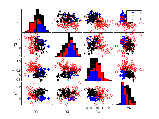
 Generate 3 groups in 4 dimensions.
Generate 3 groups in 4 dimensions.Use a maximum overlap equal to 0.15.
rng(10,'twister')
out=MixSim(3,4)
n=200;
[X,id]=simdataset(n, out.Pi, out.Mu, out.S);
spmplot(X,id)
out =

  struct with fields:

    OmegaMap: [3×3 double]
    BarOmega: 0.09
    MaxOmega: 0.15
    StdOmega: 0.05
        fail: 0
          Pi: [3×1 double]
          Mu: [3×4 double]
           S: [4×4×3 double]
       rcMax: [2×1 double]


ans(:,:,1) =

         -1.00         19.06         22.03         25.03
         16.02         -1.00         23.03         26.02
         17.03         20.03         -1.00         27.02
         18.02         21.03         24.03         -1.00


ans(:,:,2) =

         -1.00         31.02         34.02         37.02
         28.02         -1.00         35.02         38.02
         29.02         32.02         -1.00         39.02
         30.02         33.02         36.02         -1.00


ans(:,:,3) =

             0         43.02         46.01         49.01
         40.02             0         47.01         50.01
         41.02         44.02             0         51.01
         42.02         45.01         48.01             0
Related Examples
Input Arguments
Output Arguments
More About
References
Maitra, R. and Melnykov, V. (2010), Simulating data to study performance of finite mixture modeling and clustering algorithms, "The Journal of Computational and Graphical Statistics", Vol. 19, pp. 354-376. [to refer to this publication we will use "MM2010 JCGS"]
Melnykov, V., Chen, W.-C. and Maitra, R. (2012), MixSim: An R Package for Simulating Data to Study Performance of Clustering Algorithms, "Journal of Statistical Software", Vol. 51, pp. 1-25.
Davies, R. (1980), The distribution of a linear combination of chi-square random variables, "Applied Statistics", Vol. 29, pp. 323-333.
Garcia-Escudero, L.A., Gordaliza, A., Matran, C. and Mayo-Iscar, A. (2008), A General Trimming Approach to Robust Cluster Analysis. Annals of Statistics, Vol. 36, 1324-1345.
Riani, M., Cerioli, A., Perrotta, D. and Torti, F. (2015), Simulating mixtures of multivariate data with fixed cluster overlap in FSDA, "Advances in data analysis and classification", Vol. 9, pp. 461-481.
Parlett, B.N. and Reinsch, C. (1971), Balancing a Matrix for Calculation of Eigenvalues and Eigenvectors, in Bauer, F.L. Eds, "Handbook for Automatic Computation", Vol. 2, pp. 315-326, Springer.
See Also
tkmeans
|
tclust
|
tclustreg
|
lga
|
rlga
|
ncx2mixtcdf
|
restreigen