moonplot

moonplot draws the Correspondence Analysis (CA) moonplot.

expand all in page

Syntax

moonplot(out)example
moonplot(out,Name,Value)example

Description

example

moonplot(out) moonplot with all the default options.

example

moonplot(out, Name, Value) moonplot with option changedimsign.

Examples

expand all

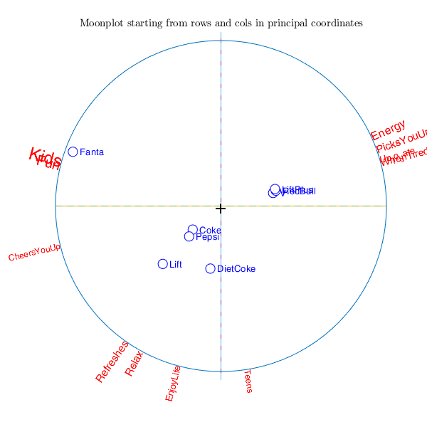
moonplot with all the default options.

Prepare the data.

load('csdPerceptions')
N=csdPerceptions;
out=CorAna(N,'plots',0);
moonplot(out);

Summary
             Singular_value    Inertia    Accounted_for    Cumulative
             ______________    _______    _____________    __________

    dim_1         0.54          0.29          0.78            0.78   
    dim_2         0.25          0.06          0.17            0.95   
    dim_3         0.11          0.01          0.03            0.98   
    dim_4         0.09          0.01          0.02            1.00   
    dim_5         0.02          0.00          0.00            1.00   
    dim_6         0.01          0.00          0.00            1.00   
    dim_7         0.01          0.00          0.00            1.00   

ROW POINTS
Results for dimension: 1
                Scores    CntrbPnt2In    CntrbDim2In
                ______    ___________    ___________

    Coke        -0.24        0.05           0.52    
    V            0.45        0.14           0.93    
    RedBull      0.47        0.14           0.92    
    LiftPlus     0.46        0.08           0.90    
    DietCoke    -0.09        0.00           0.02    
    Fanta       -1.27        0.54           0.88    
    Lift        -0.50        0.03           0.34    
    Pepsi       -0.27        0.01           0.36    

Results for dimension: 2
                Scores    CntrbPnt2In    CntrbDim2In
                ______    ___________    ___________

    Coke        -0.20        0.17           0.36    
    V            0.11        0.04           0.06    
    RedBull      0.13        0.05           0.07    
    LiftPlus     0.15        0.04           0.09    
    DietCoke    -0.54        0.16           0.76    
    Fanta        0.47        0.33           0.12    
    Lift        -0.50        0.15           0.34    
    Pepsi       -0.26        0.06           0.33    

COLUMN POINTS
Results for dimension: 1
                   Scores    CntrbPnt2In    CntrbDim2In
                   ______    ___________    ___________

    Kids           -1.32        0.43           0.92    
    Teens           0.04        0.00           0.02    
    EnjoyLife      -0.08        0.00           0.06    
    PicksYouUp      0.49        0.10           0.88    
    Refreshes      -0.29        0.02           0.21    
    CheersYouUp    -0.24        0.01           0.83    
    Energy          0.60        0.14           0.81    
    Up_to_date      0.29        0.03           0.88    
    Fun            -0.92        0.20           0.92    
    WhenTired       0.45        0.07           0.93    
    Relax          -0.25        0.01           0.20    

Results for dimension: 2
                   Scores    CntrbPnt2In    CntrbDim2In
                   ______    ___________    ___________

    Kids            0.37        0.15           0.07    
    Teens          -0.24        0.16           0.65    
    EnjoyLife      -0.29        0.13           0.79    
    PicksYouUp      0.18        0.06           0.11    
    Refreshes      -0.42        0.16           0.44    
    CheersYouUp    -0.06        0.00           0.05    
    Energy          0.27        0.14           0.17    
    Up_to_date      0.08        0.01           0.07    
    Fun             0.23        0.06           0.06    
    WhenTired       0.12        0.02           0.07    
    Relax          -0.45        0.11           0.67    

-----------------------------------------------------------
Overview ROW POINTS
                Mass    Score_1    Score_2    Inertia    CntrbPnt2In_1    CntrbPnt2In_2    CntrbDim2In_1    CntrbDim2In_2
                ____    _______    _______    _______    _____________    _____________    _____________    _____________

    Coke        0.27     -0.24      -0.20      0.03          0.05             0.17             0.52             0.36     
    V           0.21      0.45       0.11      0.05          0.14             0.04             0.93             0.06     
    RedBull     0.18      0.47       0.13      0.04          0.14             0.05             0.92             0.07     
    LiftPlus    0.11      0.46       0.15      0.03          0.08             0.04             0.90             0.09     
    DietCoke    0.04     -0.09      -0.54      0.01          0.00             0.16             0.02             0.76     
    Fanta       0.10     -1.27       0.47      0.18          0.54             0.33             0.88             0.12     
    Lift        0.04     -0.50      -0.50      0.03          0.03             0.15             0.34             0.34     
    Pepsi       0.06     -0.27      -0.26      0.01          0.01             0.06             0.36             0.33     

Overview COLUMN POINTS
                   Mass    Score_1    Score_2    Inertia    CntrbPnt2In_1    CntrbPnt2In_2    CntrbDim2In_1    CntrbDim2In_2
                   ____    _______    _______    _______    _____________    _____________    _____________    _____________

    Kids           0.07     -1.32       0.37      0.14          0.43             0.15             0.92             0.07     
    Teens          0.18      0.04      -0.24      0.02          0.00             0.16             0.02             0.65     
    EnjoyLife      0.10     -0.08      -0.29      0.01          0.00             0.13             0.06             0.79     
    PicksYouUp     0.12      0.49       0.18      0.03          0.10             0.06             0.88             0.11     
    Refreshes      0.06     -0.29      -0.42      0.02          0.02             0.16             0.21             0.44     
    CheersYouUp    0.06     -0.24      -0.06      0.00          0.01             0.00             0.83             0.05     
    Energy         0.12      0.60       0.27      0.05          0.14             0.14             0.81             0.17     
    Up_to_date     0.09      0.29       0.08      0.01          0.03             0.01             0.88             0.07     
    Fun            0.07     -0.92       0.23      0.06          0.20             0.06             0.92             0.06     
    WhenTired      0.09      0.45       0.12      0.02          0.07             0.02             0.93             0.07     
    Relax          0.03     -0.25      -0.45      0.01          0.01             0.11             0.20             0.67     

-----------------------------------------------------------
Legend
CntrbPnt2In = relative contribution of points to explain total Inertia of the latent dimension
              The sum of the numbers in a column is equal to 1
CntrbDim2In = relative contribution of latent dimension to explain total Inertia of a point
              CntrbDim2In_1+CntrbDim2In_2+...+CntrbDim2In_K=1

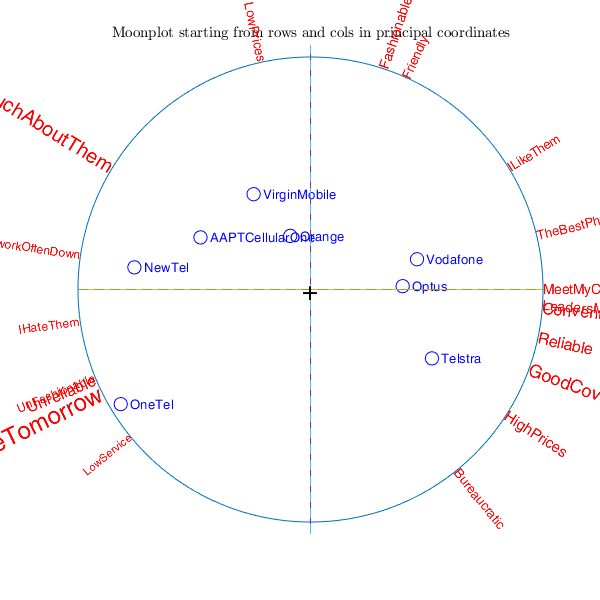
Click here for the graphical output of this example (link to Ro.S.A. website).

moonplot with option changedimsign.

Prepare the data.

load mobilephone
out=CorAna(mobilephone,'plots',0);
% Use of option changedimsign
moonplot(out,'changedimsign',[true false])

Summary
             Singular_value    Inertia    Accounted_for    Cumulative
             ______________    _______    _____________    __________

    dim_1         0.48          0.23          0.66            0.66   
    dim_2         0.25          0.06          0.19            0.84   
    dim_3         0.20          0.04          0.12            0.96   
    dim_4         0.09          0.01          0.02            0.98   
    dim_5         0.06          0.00          0.01            1.00   
    dim_6         0.03          0.00          0.00            1.00   
    dim_7         0.02          0.00          0.00            1.00   

ROW POINTS
Results for dimension: 1
                       Scores    CntrbPnt2In    CntrbDim2In
                       ______    ___________    ___________

    AAPTCellularOne     0.44        0.07           0.58    
    NewTel              0.70        0.19           0.83    
    OneTel              0.76        0.29           0.68    
    Optus              -0.37        0.10           0.80    
    Orange              0.08        0.00           0.07    
    Telstra            -0.48        0.20           0.63    
    VirginMobile        0.23        0.02           0.24    
    Vodafone           -0.42        0.12           0.76    

Results for dimension: 2
                       Scores    CntrbPnt2In    CntrbDim2In
                       ______    ___________    ___________

    AAPTCellularOne     0.21        0.06           0.13    
    NewTel              0.09        0.01           0.01    
    OneTel             -0.46        0.38           0.25    
    Optus               0.01        0.00           0.00    
    Orange              0.21        0.07           0.49    
    Telstra            -0.27        0.22           0.20    
    VirginMobile        0.38        0.22           0.66    
    Vodafone            0.12        0.03           0.06    

COLUMN POINTS
Results for dimension: 1
                                    Scores    CntrbPnt2In    CntrbDim2In
                                    ______    ___________    ___________

    Bureaucratic                    -0.21        0.01           0.22    
    LowService                       0.13        0.00           0.48    
    Friendly                        -0.13        0.00           0.13    
    LowPrices                        0.07        0.00           0.02    
    Fashionable                     -0.13        0.00           0.06    
    UnFashionable                    0.26        0.02           0.55    
    Reliable                        -0.54        0.06           0.92    
    HereTodayGoneTomorrow            1.18        0.26           0.76    
    GoodCoverage                    -0.73        0.10           0.82    
    NetworkOftenDown                 0.23        0.02           0.78    
    TheBestPhones                   -0.33        0.02           0.82    
    ConvenientlyLocatedStores       -0.63        0.09           0.92    
    HighPrices                      -0.41        0.03           0.43    
    Unreliable                       0.59        0.08           0.81    
    MeetMyCommunicationNeeds        -0.38        0.03           0.89    
    LeadersMobilePhoneTechnology    -0.43        0.04           0.97    
    ILikeThem                       -0.24        0.01           0.57    
    IHateThem                        0.28        0.03           0.95    
    DonotKnowMuchAboutThem           0.82        0.18           0.58    

Results for dimension: 2
                                    Scores    CntrbPnt2In    CntrbDim2In
                                    ______    ___________    ___________

    Bureaucratic                    -0.26        0.06           0.33    
    LowService                      -0.11        0.01           0.31    
    Friendly                         0.29        0.07           0.63    
    LowPrices                        0.33        0.09           0.52    
    Fashionable                      0.39        0.12           0.56    
    UnFashionable                   -0.10        0.01           0.09    
    Reliable                        -0.12        0.01           0.04    
    HereTodayGoneTomorrow           -0.58        0.22           0.18    
    GoodCoverage                    -0.27        0.05           0.11    
    NetworkOftenDown                 0.03        0.00           0.02    
    TheBestPhones                    0.08        0.00           0.05    
    ConvenientlyLocatedStores       -0.05        0.00           0.01    
    HighPrices                      -0.26        0.04           0.18    
    Unreliable                      -0.25        0.05           0.14    
    MeetMyCommunicationNeeds         0.00        0.00           0.00    
    LeadersMobilePhoneTechnology    -0.03        0.00           0.00    
    ILikeThem                        0.15        0.02           0.22    
    IHateThem                       -0.04        0.00           0.02    
    DonotKnowMuchAboutThem           0.50        0.25           0.22    

-----------------------------------------------------------
Overview ROW POINTS
                       Mass    Score_1    Score_2    Inertia    CntrbPnt2In_1    CntrbPnt2In_2    CntrbDim2In_1    CntrbDim2In_2
                       ____    _______    _______    _______    _____________    _____________    _____________    _____________

    AAPTCellularOne    0.09      0.44       0.21      0.03          0.07             0.06             0.58             0.13     
    NewTel             0.09      0.70       0.09      0.05          0.19             0.01             0.83             0.01     
    OneTel             0.12      0.76      -0.46      0.10          0.29             0.38             0.68             0.25     
    Optus              0.17     -0.37       0.01      0.03          0.10             0.00             0.80             0.00     
    Orange             0.10      0.08       0.21      0.01          0.00             0.07             0.07             0.49     
    Telstra            0.19     -0.48      -0.27      0.07          0.20             0.22             0.63             0.20     
    VirginMobile       0.10      0.23       0.38      0.02          0.02             0.22             0.24             0.66     
    Vodafone           0.15     -0.42       0.12      0.04          0.12             0.03             0.76             0.06     

Overview COLUMN POINTS
                                    Mass    Score_1    Score_2    Inertia    CntrbPnt2In_1    CntrbPnt2In_2    CntrbDim2In_1    CntrbDim2In_2
                                    ____    _______    _______    _______    _____________    _____________    _____________    _____________

    Bureaucratic                    0.05     -0.21      -0.26      0.01          0.01             0.06             0.22             0.33     
    LowService                      0.06      0.13      -0.11      0.00          0.00             0.01             0.48             0.31     
    Friendly                        0.05     -0.13       0.29      0.01          0.00             0.07             0.13             0.63     
    LowPrices                       0.05      0.07       0.33      0.01          0.00             0.09             0.02             0.52     
    Fashionable                     0.05     -0.13       0.39      0.01          0.00             0.12             0.06             0.56     
    UnFashionable                   0.06      0.26      -0.10      0.01          0.02             0.01             0.55             0.09     
    Reliable                        0.05     -0.54      -0.12      0.02          0.06             0.01             0.92             0.04     
    HereTodayGoneTomorrow           0.04      1.18      -0.58      0.08          0.26             0.22             0.76             0.18     
    GoodCoverage                    0.04     -0.73      -0.27      0.03          0.10             0.05             0.82             0.11     
    NetworkOftenDown                0.07      0.23       0.03      0.00          0.02             0.00             0.78             0.02     
    TheBestPhones                   0.05     -0.33       0.08      0.01          0.02             0.00             0.82             0.05     
    ConvenientlyLocatedStores       0.05     -0.63      -0.05      0.02          0.09             0.00             0.92             0.01     
    HighPrices                      0.04     -0.41      -0.26      0.02          0.03             0.04             0.43             0.18     
    Unreliable                      0.05      0.59      -0.25      0.02          0.08             0.05             0.81             0.14     
    MeetMyCommunicationNeeds        0.05     -0.38       0.00      0.01          0.03             0.00             0.89             0.00     
    LeadersMobilePhoneTechnology    0.05     -0.43      -0.03      0.01          0.04             0.00             0.97             0.00     
    ILikeThem                       0.05     -0.24       0.15      0.01          0.01             0.02             0.57             0.22     
    IHateThem                       0.08      0.28      -0.04      0.01          0.03             0.00             0.95             0.02     
    DonotKnowMuchAboutThem          0.06      0.82       0.50      0.07          0.18             0.25             0.58             0.22     

-----------------------------------------------------------
Legend
CntrbPnt2In = relative contribution of points to explain total Inertia of the latent dimension
              The sum of the numbers in a column is equal to 1
CntrbDim2In = relative contribution of latent dimension to explain total Inertia of a point
              CntrbDim2In_1+CntrbDim2In_2+...+CntrbDim2In_K=1

Input Arguments

expand all

`out` — Structure containing the output of function CorAna. Structure.

Structure containing the following fields.

Value	Description
`Lr`	cell of length $I$ containing the labels of active rows (i.e. the rows which participated to the fit).
`Lc`	cell of length $J$ containing the labels of active columns (i.e. the columns which participated to the fit).
`n`	Grand total. out.n is equal to sum(sum(out.N)). This is the number of observations.
`Dr`	Square matrix of size $I$ containing on the diagonal the row masses. This is matrix $D_r$ . $D_r=diag(r)$
`Dc`	Square matrix of size $J$ containing on the diagonal the column masses. This is matrix $D_c$ . $D_c=diag(c)$
`InertiaExplained`	matrix with 4 columnn. - First column contains the singular values (the sum of the squared singular values is the total inertia). - Second column contains the eigenvalues (the sum of the eigenvalues is the total inertia). - Third column contains the variance explained by each latent dimension. - Fourth column contains the cumulative variance explained by each dimension.
`LrSup`	cell containing the labels of the supplementary rows (i.e. the rows whicg did not participate to the fit).
`LcSup`	cell containing the labels of supplementary columns (i.e. the columns which did not participate to the fit).
`SupRowsN`	matrix of size length(LrSup)-by-c referred to supplementary rows. If there are no supplementary rows this field is not present.
`SupColsN`	matlab of size r-by-length(LcSup) referred to supplementary columns. If there are no supplementary columns this field is not present.
`RowsPriSup`	Principal coordinates of supplementary rows. If there are no supplementary rows this field is not present.
`RowsStaSup`	Standard coordinates of supplementary rows. If there are no supplementary rows this field is not present.
`RowsSymSup`	Symmetrical coordinates of supplementary rows. If there are no supplementary rows this field is not present.
`ColsPriSup`	Principal coordinates of supplementary columns. If there are no supplementary columns this field is not present.
`ColsStaSup`	Standard coordinates of of supplementary columns. If there are no supplementary columns this field is not present.
`ColsSymSup`	Symmetrical coordinates of supplementary columns. If there are no supplementary columns this field is not present.

Data Types: struct

Name-Value Pair Arguments

Specify optional comma-separated pairs of Name,Value arguments. Name is the argument name and Value is the corresponding value. Name must appear inside single quotes (' '). You can specify several name and value pair arguments in any order as Name1,Value1,...,NameN,ValueN.

Example:

 'plots',plots=struct; plots.colorcols='k'
, 'addx',0.01
, 'addy',0.01
, 'changedimsign', [true false]
, 'xlimx',[-1 1]
, 'ylimy',[0 1]
, 'd1',2
, 'd2',3
,'h',h1 where h1=subplot(2,1,1)

`plots` —Customize plot appearance.scalar | structure.

If plots is not a structure, a plot which shows the Principal coordinates of rows and columns is shown on the screen. If plots is a structure it may contain the following fields:

Value	Description
`alpha`	type of plot, scalar in the interval [0 1] or a string identifying the type of coordinates to use in the plot. If $plots.alpha='rowprincipal'$ the row points are in principal coordinates and the column coordinates are standard coordinates. Distances between row points are (approximated) chi-squared distances (row-metric-preserving). The position of the row points are at the weighted average of the column points. Note that 'rowprincipal' can also be specified setting plots.alpha=1. If $plots.alpha='colprincipal'$ , the column coordinates are referred to as principal coordinates and the row coordinates as standard coordinates. Distances between column points are (approximated) chi-squared distances (column-metric-preserving). The position of the column points are at the weighted average of the row points. Note that 'colprincipal' can also be specified setting plots.alpha=0. If $plots.alpha='symbiplot'$ , the row and column coordinates are scaled similarly. The sum of weighted squared coordinates for each dimension is equal to the corresponding singular values. These coordinates are often called symmetrical coordinates. This representation is particularly useful if one is primarily interested in the relationships between categories of row and column variables rather than in the distances among rows or among columns. 'symbiplot' can also be specified setting plots.alpha=0.5; If $plots.alpha='bothprincipal'$ , both the rows and columns are depicted in principal coordinates. Such a plot is often referred to as a symmetrical plot or French symemtrical model. Note that such a symmetrical plot does not provide a feasible solution in the sense that it does not approximate matrix $D_r^{-0.5}(P-rc')D_c^{-0.5}$ . If $plots.alpha='bothstandard'$ , both the rows and columns are depicted in standard coordinates. If $plots.alpha='rowgab'$ , rows are in principal coordinates and columns are in standard coordinates multiplied by the mass. This biplot has been suggested by Gabriel and Odoroff (1990). If $plots.alpha='colgab'$ , columns are in principal coordinates and rows are in standard coordinates multiplied by the mass. This biplot has been suggested by Gabriel and Odoroff (1990). If $plots.alpha='rowgreen'$ , rows are in principal coordinates and columns are in standard coordinates multiplied by square root of the mass. This biplot has been suggested by Greenacre and incorporates the contribution of points. In this display, points that contribute very little to the solution, are close to the center of the biplot and are relatively unimportant to the interpretation. This biplot is often referred as contribution biplot because it visually shows the most contributing points (Greenacre 2006b). If $plots.alpha='colgreen'$ , columns in principal coordinates and rows in standard coordinates multiplied by the square root of the mass. This biplot has been suggested by Greenacre and incorporates the contribution of points. In this display, points that contribute very little to the solution, are close to the center of the biplot and are relatively unimportant to the interpretation. This biplot is often referred as contribution biplot because it shows visually the most contributing points (Greenacre 2006b). If $plots.alpha=scalar$ in the interval [0 1], row coordinates are given by $D_r^{-1/2} U \Gamma^\alpha$ and column coordinates are given by $D_c^{-1/2} V \Gamma^{1-\alpha}$ . Note that for any choice of $\alpha$ the matrix product $D_r^{-1/2} U \Gamma^\alpha (D_c^{-1/2} V \Gamma^{1-\alpha})^T$ optimally approximates matrix $D_r^{-0.5}(P-rc')D_c^{-0.5}$ , in the sense that the sum of squared differences between $D_r^{1/2} D_r^{-1/2} U \Gamma^\alpha (D_c^{-1/2} V \Gamma^{1-\alpha})^T D_c^{1/2}$ and $D_r^{-0.5}(P-rc')D_c^{-0.5}$ is as small as possible.
`FontSize`	scalar which specifies the font size of row labels. The default value is 10.
`FontSizeSup`	scalar which specifies the font size of row labels of supplementary points. The default value is 10.
`MarkerSize`	scalar which specifies the marker size of symbols associated with rows. The default value is 10.
`SymbolRows`	character which specifies the symbol to use for row points. If this field is not present the default symbols is 'o'.
`SymbolRowsSup`	character which specifies the symbol to use for supplementary row points. If this field is not present the default symbols is 'o'.
`ColorRows`	character which specifies the symbol to use for row points or RGB triplet. If this field is not present the default color is 'b'.
`ColorCols`	character which specifies the symbol to use for column points or RGB triplet. If this field is not present the default color is 'r'.
`ColorRowsSup`	character which specifies the symbol to use for row points or RGB triplet. If this field is not present the default color is 'b'.
`ColorColsSup`	character which specifies the symbol to use for supplementary column points or RGB triplet. If this field is not present the default color is 'r'.
`MarkerFaceColorRows`	character which specifies the marker fill color to use for active row points or RGB triplet. If this field is not present the default color is 'auto'.
`MarkerFaceColorRowsSup`	character which specifies the marker fill color to use for supplementary row points or RGB triplet. If this field is not present the default color is 'auto'.

Example: 'plots',plots=struct; plots.colorcols='k'

Data Types: double

`addx` —horizontal displacement for labels.scalar.

Amount of horizontal displacement which has been put on the labels in the plot. The defalut value of addx is 0.04.

Example: 'addx',0.01

Data Types: double

`addy` —vertical displacement for labels.scalar.

Amount of vertical displacement which has been put on the labels in the plot. The defalut value of addy is 0.

Example: 'addy',0.01

Data Types: double

`changedimsign` —change chosen dimension sign.boolean vector of length 2.

Sometimes for better interpretability it is necessary to change the sign of the coordinates for the chosen dimension. If changedimsign(1) is true the sign of the coordinates for first chosen dimension is changed. If changedimsign(2) is true the sign of the coordinates for first chosen dimension is changed. As default the dimensions are the first and the second however, they can be changed using option plots.dim. The defaul value of changedimsign is [false false] that is the sign is not changed.

Example: 'changedimsign', [true false]

Data Types: boolean

`xlimx` —Min and Max of the x axis.vector.

Vector with two elements controlling minimum and maximum of the x axis.

Example: 'xlimx',[-1 1]

Data Types: double

`ylimy` —Min and Max of the y axis.vector.

Vector with two elements controlling minimum and maximum of the y axis.

Example: 'ylimy',[0 1]

Data Types: double

`d1` —Dimension to show on the horizontal axis.positive integer.

Positive integer in the range 1, 2, .., K which indicates the dimension to show on the x axis. The default value of d1 is 1.

Example: 'd1',2

Data Types: single | double

`d2` —Dimension to show on the vertical axis.positive integer.

Positive integer in the range 1, 2, .., K which indicates the dimension to show on the y axis. The default value of d2 is 2.

Example: 'd2',3

Data Types: single | double

`h` —the axis handle of a figure where to send the moonplot.this can be used to host the moonplot in a subplot of a complex figure formed by different panels (for example a panel with moonplot from plots.

alpha=0.2 and another with moonplot from plots.alpha=0.5).

Example: 'h',h1 where h1=subplot(2,1,1)

Data Types: Axes object (supplied as a scalar)

Output Arguments

expand all

References

Benzecri, J.-P. (1992), "Correspondence Analysis Handbook", New-York, Dekker.

Benzecri, J.-P. (1980), "L'analyse des donnees tome 2: l'analyse des correspondances", Paris, Bordas.

Greenacre, M.J. (1993), "Correspondence Analysis in Practice", London, Academic Press.

Bock, T. (2011), Improving the display of correspondence analysis using moon plots, "International Journal of Market Research", Vol. 53, pp. 307-326.

Gabriel, K.R. and Odoroff, C. (1990), Biplots in biomedical research, "Statistics in Medicine", Vol. 9, pp. 469-485.

Greenacre, M.J. (1993), Biplots in correspondence Analysis, "Journal of Applied Statistics", Vol. 20, pp. 251-269.

Documentation

moonplot

Syntax

Description

Examples

moonplot with all the default options.

moonplot with option changedimsign.

Input Arguments

`out` — Structure containing the output of function CorAna. Structure.

Name-Value Pair Arguments

`plots` —Customize plot appearance.scalar | structure.

`addx` —horizontal displacement for labels.scalar.

`addy` —vertical displacement for labels.scalar.

`changedimsign` —change chosen dimension sign.boolean vector of length 2.

`xlimx` —Min and Max of the x axis.vector.

`ylimy` —Min and Max of the y axis.vector.

`d1` —Dimension to show on the horizontal axis.positive integer.

`d2` —Dimension to show on the vertical axis.positive integer.

`h` —the axis handle of a figure where to send the moonplot.this can be used to host the moonplot in a subplot of a complex figure formed by different panels (for example a panel with moonplot from plots.

Output Arguments

References

See Also

Documentation

moonplot

Syntax

Description

Examples

moonplot with all the default options.

moonplot with option changedimsign.

Input Arguments

out — Structure containing the output of function CorAna. Structure.

Name-Value Pair Arguments

plots —Customize plot appearance.scalar | structure.

addx —horizontal displacement for labels.scalar.

addy —vertical displacement for labels.scalar.

changedimsign —change chosen dimension sign.boolean vector of length 2.

xlimx —Min and Max of the x axis.vector.

ylimy —Min and Max of the y axis.vector.

d1 —Dimension to show on the horizontal axis.positive integer.

d2 —Dimension to show on the vertical axis.positive integer.

h —the axis handle of a figure where to send the moonplot.this can be used to host the moonplot in a subplot of a complex figure formed by different panels (for example a panel with moonplot from plots.

Output Arguments

References

See Also

`out` — Structure containing the output of function CorAna. Structure.

`plots` —Customize plot appearance.scalar | structure.

`addx` —horizontal displacement for labels.scalar.

`addy` —vertical displacement for labels.scalar.

`changedimsign` —change chosen dimension sign.boolean vector of length 2.

`xlimx` —Min and Max of the x axis.vector.

`ylimy` —Min and Max of the y axis.vector.

`d1` —Dimension to show on the horizontal axis.positive integer.

`d2` —Dimension to show on the vertical axis.positive integer.

`h` —the axis handle of a figure where to send the moonplot.this can be used to host the moonplot in a subplot of a complex figure formed by different panels (for example a panel with moonplot from plots.