simdataset
simdataset simulates and-or contaminates a dataset given the parameters of a finite mixture model with Gaussian components
Syntax
Description
simdataset(n, Pi, Mu, S) generates a matrix of size -by-p containing n observations p dimensions from k groups. More precisely, this function produces a dataset of n observations from a mixture model with parameters 'Pi' (mixing proportions), 'Mu' (mean vectors), and 'S' (covariance matrices). Mixture component sample sizes are produced as a realization from a multinomial distribution with probabilities given by the mixing proportions. For example, if n=200, k=4 and Pi=[0.25, 0.25, 0.25, 0.25] function Nk1=mnrnd( n-k, Pi) is used to generate k integers (whose sum is n-k) from the multinomial distribution with parameters n-k and Pi. The size of the groups is given by Nk1+1. The first Nk1(1)+1 observations are generated using centroid Mu(1,:) and covariance S(:,:,1), ..., the last Nk1(k)+1 observations are generated using centroid Mu(k,:) and covariance S(:,:,k).
DETAILS.
To make a dataset more challenging for clustering, a user might want to simulate noise variables or outliers. The optional parameter 'noiseunits' controls the number and the type of outliers which must be added. The optional parameter 'noisevars' controls the number and the type of noise variables which must be added (it is possible to control the distribution, the interval and the number). Finally, the user can apply an inverse Box-Cox transformation providing a vector of coefficients 'lambda'. The value 1 implies that no transformation is needed for the corresponding coordinate. It is also possible to add outliers to an existing dataset by simply suppling as first argument the matrix of existing data.
Examples
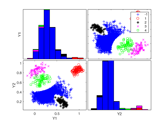
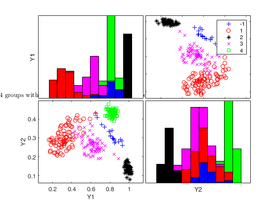
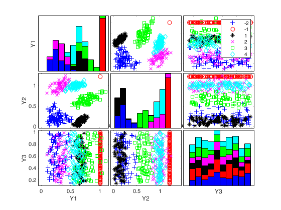
 Generate 4 groups in 2 dimensions and add outliers from uniform distribution.
Generate 4 groups in 2 dimensions and add outliers from uniform distribution.
rng('default')
rng(100)
out = MixSim(4,2,'BarOmega',0.01);
n=300;
noisevars=0;
noiseunits=3000;
[X,id]=simdataset(n, out.Pi, out.Mu, out.S,'noisevars',noisevars,'noiseunits',noiseunits);
spmplot(X,id);
title('4 groups with outliers from uniform')
Related Examples
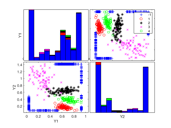
Add outliers generated from Chi2 with 5 degrees of freedom.
Add outliers generated from Chi2 with 5 degrees of freedom.
out = MixSim(4,2,'BarOmega',0.01);
n=300;
noisevars=0;
noiseunits=struct;
noiseunits.number=3000;
% Add asymmetric very concentrated noise
noiseunits.typeout={'Chisquare5'};
[X,id]=simdataset(n, out.Pi, out.Mu, out.S,'noisevars',noisevars,'noiseunits',noiseunits);
spmplot(X,id);
title('4 groups with outliers from $\chi^2_5$','Interpreter','Latex')
Add outliers generated from Chi2 with 40 degrees of freedom.
Add outliers generated from Chi2 with 40 degrees of freedom.
n=300;
out = MixSim(4,2,'BarOmega',0.01);
noisevars=0;
noiseunits=struct;
noiseunits.number=3000;
% Add asymmetric concentrated noise
noiseunits.typeout={'Chisquare40'};
[X,id]=simdataset(n, out.Pi, out.Mu, out.S,'noisevars',noisevars,'noiseunits',noiseunits);
spmplot(X,id);
title('4 groups with outliers from $\chi^2_{40}$','Interpreter','Latex')
Add outliers generated from normal distribution.
Add outliers generated from normal distribution.
n=300;
out = MixSim(4,2,'BarOmega',0.01);
noisevars=0;
noiseunits=struct;
noiseunits.number=3000;
% Add normal noise
noiseunits.typeout={'normal'};
[X,id]=simdataset(n, out.Pi, out.Mu, out.S,'noisevars',noisevars,'noiseunits',noiseunits);
spmplot(X,id);
title('4 groups with outliers from normal distribution','Interpreter','Latex')
Add outliers generated from Student T with 5 degrees of freedom.
Add outliers generated from Student T with 5 degrees of freedom.
n=300;
out = MixSim(4,2,'BarOmega',0.01);
noisevars=0;
noiseunits=struct;
noiseunits.number=3000;
% Add outliers from T5
noiseunits.typeout={'T5'};
[X,id]=simdataset(n, out.Pi, out.Mu, out.S,'noisevars',noisevars,'noiseunits',noiseunits);
spmplot(X,id);
title('4 groups with outliers from Student T with 5 degrees if freedom','Interpreter','Latex')
Warning: it was not possible to generate 3000 outliers
in 30000 replicates in the interval [0.16444--1.0276]
Number of values which was possible to generate is equal to 30
Please modify the type of outliers using option 'typeout'
or increase input option 'alpha'
The value of alpha now is 0.001
Outliers have been generated according to T5
Warning: Output matrix X will have just 330 rows and not 3300
Add componentwise contamination.
Add componentwise contamination.
n=300;
out = MixSim(4,2,'BarOmega',0.01);
noisevars='';
noiseunits=struct;
noiseunits.number=3000;
% Add asymmetric concentrated noise
noiseunits.typeout={'componentwise'};
[X,id]=simdataset(n, out.Pi, out.Mu, out.S,'noisevars',noisevars,'noiseunits',noiseunits);
spmplot(X,id);
title('4 groups with component wise outliers','Interpreter','Latex')
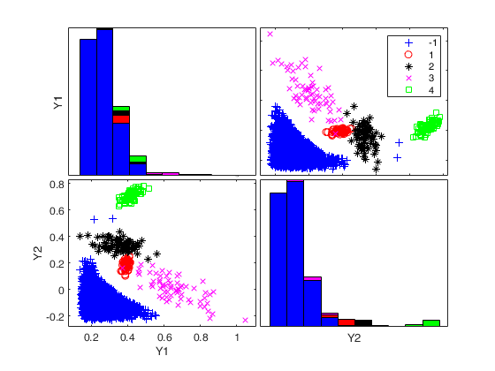
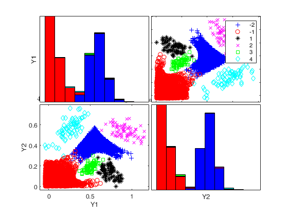
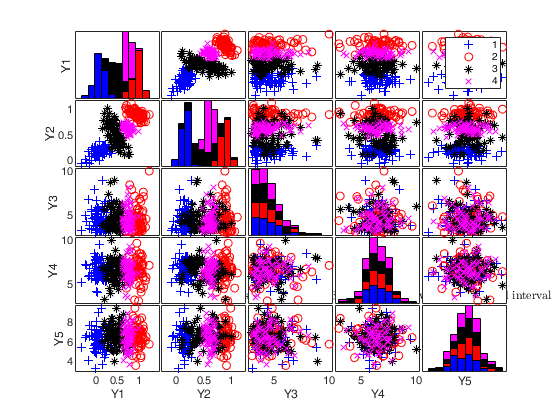
Add outliers generated from Chisquare and T distribution.
Add outliers generated from Chisquare and T distribution.
n=300;
out = MixSim(4,2,'BarOmega',0.01);
noisevars=0;
noiseunits=struct;
noiseunits.number=5000*ones(2,1);
noiseunits.typeout={'Chisquare3','T20'};
[X,id]=simdataset(n, out.Pi, out.Mu, out.S,'noisevars',noisevars,'noiseunits',noiseunits);
spmplot(X,id);
title('4 groups with outliers from $\chi^2_{3}$ and $T_{20}$','Interpreter','Latex')
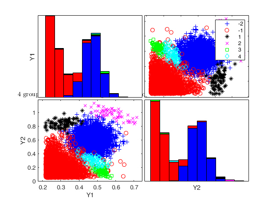
Add outliers from Chisquare and T distribution and use a personalized value of alpha.
Add outliers from Chisquare and T distribution and use a personalized value of alpha.
n=300;
out = MixSim(4,2,'BarOmega',0.01);
noisevars=0;
noiseunits=struct;
noiseunits.number=5000*ones(2,1);
noiseunits.typeout={'Chisquare3','T20'};
noiseunits.alpha=0.2;
[X,id]=simdataset(n, out.Pi, out.Mu, out.S,'noisevars',noisevars,'noiseunits',noiseunits);
spmplot(X,id);
title('4 groups with outliers from $\chi^2_{3}$ and $T_{20}$ and $\alpha=0.2$','Interpreter','Latex')
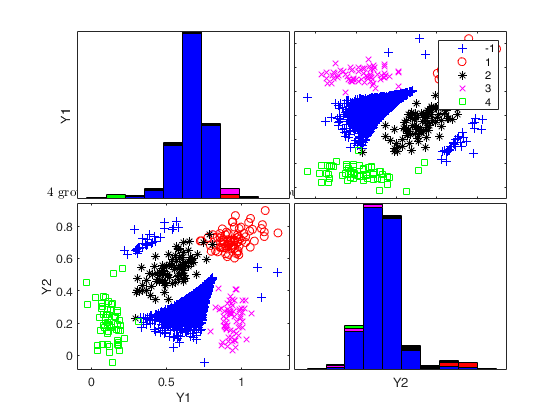
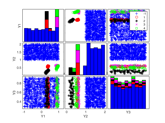
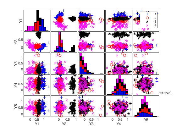
Add outliers from Chi2 and point mass contamination and add one noise variable.
Add outliers from Chi2 and point mass contamination and add one noise variable.
n=300;
out = MixSim(4,2,'BarOmega',0.01);
noisevars=struct;
noisevars.number=1;
noiseunits=struct;
noiseunits.number=[100 100];
noiseunits.typeout={'pointmass' 'Chisquare5'};
[X,id]=simdataset(n, out.Pi, out.Mu, out.S,'noisevars',noisevars,'noiseunits',noiseunits);
spmplot(X,id);
title('4 groups with outliers from $\chi^2_{5}$ and point mass $+1$ noise var','Interpreter','Latex')
Example of the use of personalized interval to generate outliers.
Example of the use of personalized interval to generate outliers.
n=300;
out = MixSim(4,2,'BarOmega',0.01);
noiseunits=struct;
noiseunits.number=1000;
noiseunits.typeout={'uniform'};
% Generate outliers in the interval [-1 1] for the first variable and
% interval [1 2] for the second variable
noiseunits.interval=[-1 1;
1 2];
% Finally add a noise variable
noisevars=struct;
noisevars.number=1;
[X,id]=simdataset(n, out.Pi, out.Mu, out.S,'noisevars',noisevars,'noiseunits',noiseunits);
spmplot(X,id);
title('4 groups with outliers from uniform using a personalized interval $+1$ noise var','Interpreter','Latex')
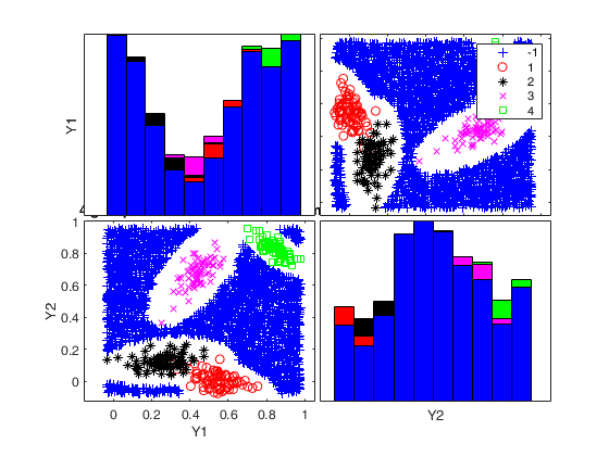
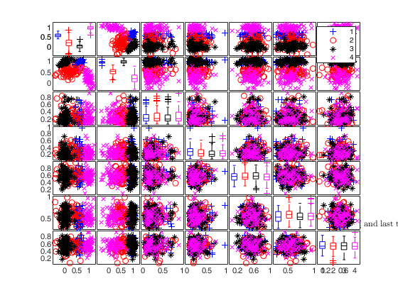
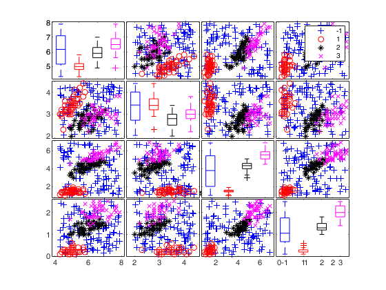
Add 5 noise variables.
Add 5 noise variables.
n=300;
out = MixSim(4,2,'BarOmega',0.01);
noisevars=struct;
noisevars.number=[2 3];
noisevars.distribution={'Chisquare3','T20'};
noiseunits='';
[X,id]=simdataset(n, out.Pi, out.Mu, out.S,'noisevars',noisevars,'noiseunits',noiseunits);
spmplot(X,id,[],'box');
title('4 groups in 2 dims with 5 noise variables. First two from $\chi^2_{3}$ and last three from $T_{20}$','Interpreter','Latex')
Add 3 noise variables.
Add 3 noise variables.
n=300;
out = MixSim(4,2,'BarOmega',0.01);
noisevars=struct;
noisevars.number=[1 2];
noisevars.distribution={'Chisquare3','T2'};
noiseunits='';
[X,id]=simdataset(n, out.Pi, out.Mu, out.S,'noisevars',noisevars,'noiseunits',noiseunits);
spmplot(X,id);
title('4 groups in 2 dims with 3 noise variables. First from $\chi^2_{3}$ and last two from $T_{2}$','Interpreter','Latex')
Add 3 noise variables and use 'minmax' interval.
Add 3 noise variables and use 'minmax' interval.
n=300;
out = MixSim(4,2,'BarOmega',0.01);
noisevars=struct;
noisevars.number=[1 2];
noisevars.distribution={'Chisquare3','T20'};
noisevars.interval='minmax';
noiseunits='';
[X,id]=simdataset(n, out.Pi, out.Mu, out.S,'noisevars',noisevars,'noiseunits',noiseunits);
spmplot(X,id);
title('4 groups in 2 dims with 3 noise variables with ''minimax'' interval','Interpreter','Latex')
Add 3 noise variables and use a personalized interval for each variable.
Add 3 noise variables and use a personalized interval for each variable.
n=300;
out = MixSim(4,2,'BarOmega',0.01);
noisevars=struct;
noisevars.number=[1 2];
noisevars.distribution={'Chisquare3','T20'};
noiseunits='';
% In this example we supply min and max for each noise variable
v1=sum(noisevars.number);
noisevars.interval=[3*ones(1,v1); 10*ones(1,v1)];
[X,id]=simdataset(n, out.Pi, out.Mu, out.S,'noisevars',noisevars,'noiseunits',noiseunits);
spmplot(X,id);
title('4 groups in 2 dims with 3 noise variables with personalized interval','Interpreter','Latex')
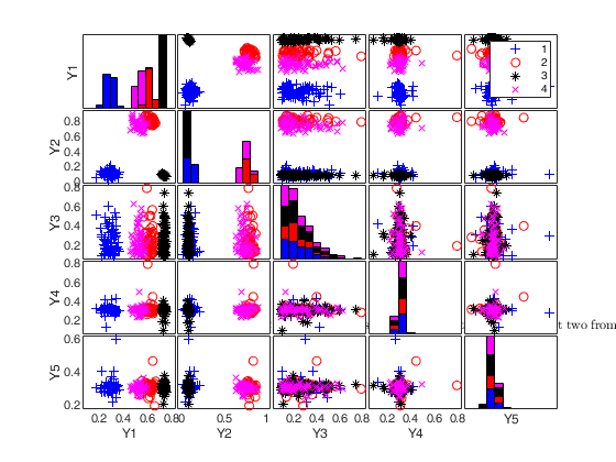
Add noise to an existing dataset.
Add noise to an existing dataset.Add outliers generated from uniform distribution to the IRIS dataset
load fisheriris;
Y=meas;
Mu=grpstats(Y,species);
S=zeros(4,4,3);
S(:,:,1)=cov(Y(1:50,:));
S(:,:,2)=cov(Y(51:100,:));
S(:,:,3)=cov(Y(101:150,:));
pigen=ones(3,1)/3;
% Add 100 outliers and specify a very small value of alpha
noisevars=0;
noiseunits=struct;
noiseunits.number=100;
noiseunits.alpha=0.000001;
% In this case the first argument which is supplied to simdataset is
% the original matrix X
[Ywithnoise,id]=simdataset(Y, pigen, Mu, S,'noisevars',noisevars,'noiseunits',noiseunits);
spmplot(Ywithnoise,id,[],'box');
title('4 groups with outliers from uniform')
Input Arguments
Output Arguments
References
Maitra, R. and Melnykov, V. (2010), Simulating data to study performance of finite mixture modeling and clustering algorithms, "The Journal of Computational and Graphical Statistics", Vol. 19, pp. 354-376. [to refer to this publication we will use "MM2010 JCGS"]
Melnykov, V., Chen, W.-C. and Maitra, R. (2012), MixSim: An R Package for Simulating Data to Study Performance of Clustering Algorithms, "Journal of Statistical Software", Vol. 51, pp. 1-25.
Davies, R. (1980), The distribution of a linear combination of chi-square random variables, "Applied Statistics", Vol. 29, pp. 323-333.
Riani, M., Cerioli, A., Perrotta, D. and Torti, F. (2015), Simulating mixtures of multivariate data with fixed cluster overlap in FSDA, "Advances in data analysis and classification", Vol. 9, pp. 461-481.