simdataset

simdataset simulates and-or contaminates a dataset given the parameters of a finite mixture model with Gaussian components

Syntax

  • X=simdataset(n, Pi, Mu, S)example
  • X=simdataset(n, Pi, Mu, S,Name,Value)example
  • [X,id]=simdataset(___)example

Description

simdataset(n, Pi, Mu, S) generates a matrix of size $n$-by-$p$ containing $n$ observations $p$ dimensions from $k$ groups. More precisely, this function produces a dataset of n observations from a mixture model with parameters 'Pi' (mixing proportions), 'Mu' (mean vectors), and 'S' (covariance matrices). Mixture component sample sizes are produced as a realization from a multinomial distribution with probabilities given by the mixing proportions. For example, if n=200, k=4 and Pi=[0.25, 0.25, 0.25, 0.25] function Nk1=mnrnd( n-k, Pi) is used to generate k integers (whose sum is n-k) from the multinomial distribution with parameters n-k and Pi. The size of the groups is given by Nk1+1. The first Nk1(1)+1 observations are generated using centroid Mu(1,:) and covariance S(:,:,1), ..., the last Nk1(k)+1 observations are generated using centroid Mu(k,:) and covariance S(:,:,k).

DETAILS.

To make a dataset more challenging for clustering, a user might want to simulate noise variables or outliers. The optional parameter 'noiseunits' controls the number and the type of outliers which must be added. The optional parameter 'noisevars' controls the number and the type of noise variables which must be added (it is possible to control the distribution, the interval and the number). Finally, the user can apply an inverse Box-Cox transformation providing a vector of coefficients 'lambda'. The value 1 implies that no transformation is needed for the corresponding coordinate. It is also possible to add outliers to an existing dataset by simply suppling as first argument the matrix of existing data.

example

X =simdataset(n, Pi, Mu, S) Example of mixture generation.

example

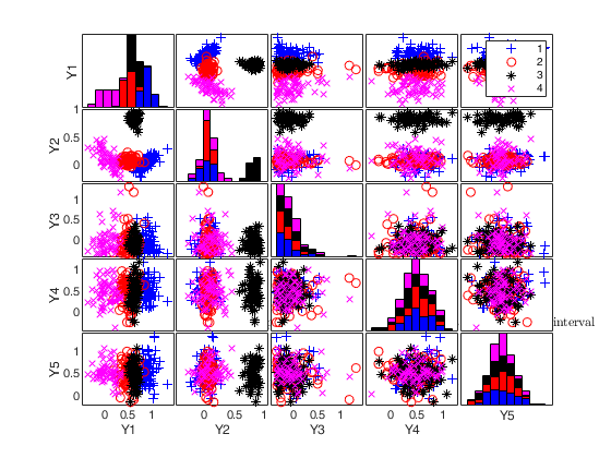
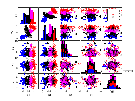
X =simdataset(n, Pi, Mu, S, Name, Value) Generate 4 groups in 2 dimensions.

example

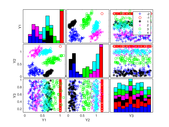
[X, id] =simdataset(___) Generate 4 groups in 2 dimensions and add outliers from uniform distribution.

Examples

expand all

  • Example of mixture generation.
  • out = MixSim(4,2,'BarOmega',0.01);
    n=60;
    [X,id]=simdataset(n, out.Pi, out.Mu, out.S);
    %  Simulate dataset with 10 outliers
    [X,id]=simdataset(n, out.Pi, out.Mu, out.S,'noiseunits',10);
    %  Simulate dataset with 100 outliers
    out = MixSim(4,3,'BarOmega',0.1);
    n=300;
    [X,id]=simdataset(n, out.Pi, out.Mu, out.S,'noiseunits',100);
    spmplot(X,id);

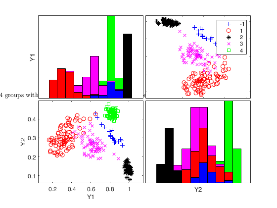
  • Generate 4 groups in 2 dimensions.
  • rng('default')
    rng(100)
    out = MixSim(4,2,'BarOmega',0.01);
    n=300;
    [X,id]=simdataset(n, out.Pi, out.Mu, out.S);
    spmplot(X,id);
    title('4 groups without noise and outliers')

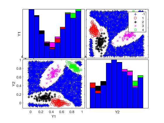
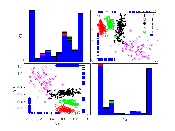
  • Generate 4 groups in 2 dimensions and add outliers from uniform distribution.
  • rng('default')
    rng(100)
    out = MixSim(4,2,'BarOmega',0.01);
    n=300;
    noisevars=0;
    noiseunits=3000;
    [X,id]=simdataset(n, out.Pi, out.Mu, out.S,'noisevars',noisevars,'noiseunits',noiseunits);
    spmplot(X,id);
    title('4 groups with outliers from uniform')
    Click here for the graphical output of this example (link to Ro.S.A. website).

    Related Examples

    expand all

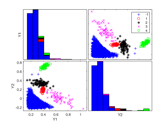
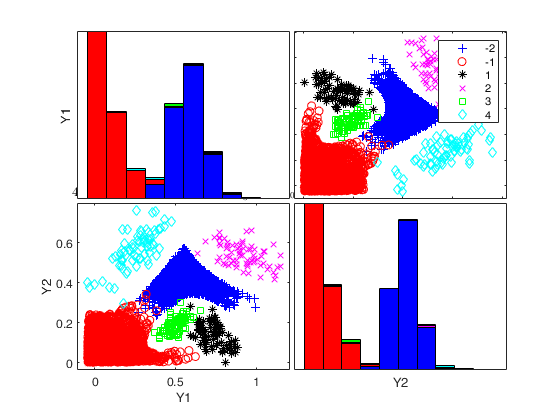
  • Add outliers generated from Chi2 with 5 degrees of freedom.
  • out = MixSim(4,2,'BarOmega',0.01);
    n=300;
    noisevars=0;
    noiseunits=struct;
    noiseunits.number=3000;
    % Add asymmetric very concentrated noise
    noiseunits.typeout={'Chisquare5'};
    [X,id]=simdataset(n, out.Pi, out.Mu, out.S,'noisevars',noisevars,'noiseunits',noiseunits);
    spmplot(X,id);
    title('4 groups with outliers from $\chi^2_5$','Interpreter','Latex')
    Click here for the graphical output of this example (link to Ro.S.A. website)

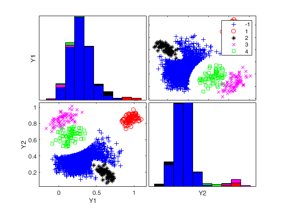
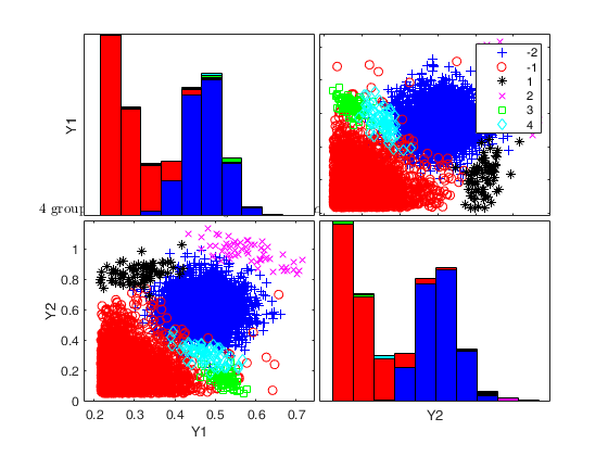
  • Add outliers generated from Chi2 with 40 degrees of freedom.
  • n=300;
    out = MixSim(4,2,'BarOmega',0.01);
    noisevars=0;
    noiseunits=struct;
    noiseunits.number=3000;
    % Add asymmetric concentrated noise
    noiseunits.typeout={'Chisquare40'};
    [X,id]=simdataset(n, out.Pi, out.Mu, out.S,'noisevars',noisevars,'noiseunits',noiseunits);
    spmplot(X,id);
    title('4 groups with outliers from $\chi^2_{40}$','Interpreter','Latex')
    Click here for the graphical output of this example (link to Ro.S.A. website)

  • Add outliers generated from normal distribution.
  • n=300;
    out = MixSim(4,2,'BarOmega',0.01);
    noisevars=0;
    noiseunits=struct;
    noiseunits.number=3000;
    % Add normal noise
    noiseunits.typeout={'normal'};
    [X,id]=simdataset(n, out.Pi, out.Mu, out.S,'noisevars',noisevars,'noiseunits',noiseunits);
    spmplot(X,id);
    title('4 groups with outliers from normal distribution','Interpreter','Latex')
    Click here for the graphical output of this example (link to Ro.S.A. website)

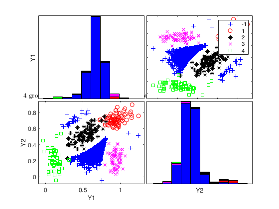
  • Add outliers generated from Student T with 5 degrees of freedom.
  • n=300;
    out = MixSim(4,2,'BarOmega',0.01);
    noisevars=0;
    noiseunits=struct;
    noiseunits.number=3000;
    % Add outliers from T5
    noiseunits.typeout={'T5'};
    [X,id]=simdataset(n, out.Pi, out.Mu, out.S,'noisevars',noisevars,'noiseunits',noiseunits);
    spmplot(X,id);
    title('4 groups with outliers from Student T with 5 degrees if freedom','Interpreter','Latex')
    Warning: it was not possible to generate 3000 outliers
    in 30000 replicates in the interval [0.16444--1.0276]
    Number of values which was possible to generate is equal to 30
    Please modify the type of outliers using option 'typeout' 
    or increase input option 'alpha'
    The value of alpha now is 0.001
    Outliers have been generated according to T5
    Warning: Output matrix X will have just 330 rows and not 3300 
    
    Click here for the graphical output of this example (link to Ro.S.A. website)

  • Add componentwise contamination.
  • n=300;
    out = MixSim(4,2,'BarOmega',0.01);
    noisevars='';
    noiseunits=struct;
    noiseunits.number=3000;
    % Add asymmetric concentrated noise
    noiseunits.typeout={'componentwise'};
    [X,id]=simdataset(n, out.Pi, out.Mu, out.S,'noisevars',noisevars,'noiseunits',noiseunits);
    spmplot(X,id);
    title('4 groups with component wise outliers','Interpreter','Latex')
    Click here for the graphical output of this example (link to Ro.S.A. website)

  • Add outliers generated from Chisquare and T distribution.
  • n=300;
    out = MixSim(4,2,'BarOmega',0.01);
    noisevars=0;
    noiseunits=struct;
    noiseunits.number=5000*ones(2,1);
    noiseunits.typeout={'Chisquare3','T20'};
    [X,id]=simdataset(n, out.Pi, out.Mu, out.S,'noisevars',noisevars,'noiseunits',noiseunits);
    spmplot(X,id);
    title('4 groups with outliers from $\chi^2_{3}$ and $T_{20}$','Interpreter','Latex')
    Click here for the graphical output of this example (link to Ro.S.A. website)

  • Add outliers from Chisquare and T distribution and use a personalized value of alpha.
  • n=300;
    out = MixSim(4,2,'BarOmega',0.01);
    noisevars=0;
    noiseunits=struct;
    noiseunits.number=5000*ones(2,1);
    noiseunits.typeout={'Chisquare3','T20'};
    noiseunits.alpha=0.2;
    [X,id]=simdataset(n, out.Pi, out.Mu, out.S,'noisevars',noisevars,'noiseunits',noiseunits);
    spmplot(X,id);
    title('4 groups with outliers from $\chi^2_{3}$ and $T_{20}$ and $\alpha=0.2$','Interpreter','Latex')
    Click here for the graphical output of this example (link to Ro.S.A. website)

  • Add outliers from Chi2 and point mass contamination and add one noise variable.
  • n=300;
    out = MixSim(4,2,'BarOmega',0.01);
    noisevars=struct;
    noisevars.number=1;
    noiseunits=struct;
    noiseunits.number=[100 100];
    noiseunits.typeout={'pointmass' 'Chisquare5'};
    [X,id]=simdataset(n, out.Pi, out.Mu, out.S,'noisevars',noisevars,'noiseunits',noiseunits);
    spmplot(X,id);
    title('4 groups with outliers from $\chi^2_{5}$ and point mass $+1$ noise var','Interpreter','Latex')
    Click here for the graphical output of this example (link to Ro.S.A. website)

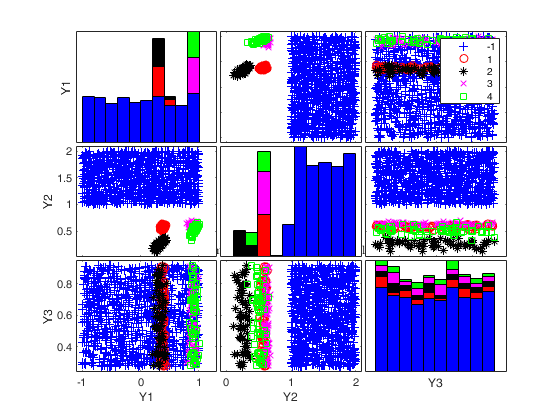
  • Example of the use of personalized interval to generate outliers.
  • n=300;
    out = MixSim(4,2,'BarOmega',0.01);
    noiseunits=struct;
    noiseunits.number=1000;
    noiseunits.typeout={'uniform'};
    % Generate outliers in the interval [-1 1] for the first variable and
    % interval [1 2] for the second variable
    noiseunits.interval=[-1 1;
    1 2];
    % Finally add a noise variable
    noisevars=struct;
    noisevars.number=1;
    [X,id]=simdataset(n, out.Pi, out.Mu, out.S,'noisevars',noisevars,'noiseunits',noiseunits);
    spmplot(X,id);
    title('4 groups with outliers from uniform using a personalized interval $+1$ noise var','Interpreter','Latex')
    Click here for the graphical output of this example (link to Ro.S.A. website)

  • Example of the use of personalized interval to generate outliers (1).
  • Generate 1000 outliers from uniform in the interval [-2 3] and 1000 units using componentwise contamination in the interval [-2 3]

    n=300;
    out = MixSim(4,2,'BarOmega',0.01);
    noiseunits=struct;
    noiseunits.number=[1000 1000];
    noiseunits.typeout={'uniform' 'componentwise'};
    noiseunits.interval=[-2 3];
    [X,id]=simdataset(n, out.Pi, out.Mu, out.S,'noiseunits',noiseunits);
    spmplot(X,id);
    title('4 groups with outliers componentwise and from uniform in interval [-2 3]','Interpreter','Latex')

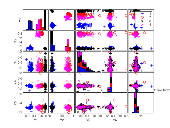
  • Add 5 noise variables.
  • n=300;
    out = MixSim(4,2,'BarOmega',0.01);
    noisevars=struct;
    noisevars.number=[2 3];
    noisevars.distribution={'Chisquare3','T20'};
    noiseunits='';
    [X,id]=simdataset(n, out.Pi, out.Mu, out.S,'noisevars',noisevars,'noiseunits',noiseunits);
    spmplot(X,id,[],'box');
    title('4 groups in 2 dims with 5 noise variables. First two from $\chi^2_{3}$ and last three from $T_{20}$','Interpreter','Latex')
    Click here for the graphical output of this example (link to Ro.S.A. website)

  • Add 3 noise variables.
  • n=300;
    out = MixSim(4,2,'BarOmega',0.01);
    noisevars=struct;
    noisevars.number=[1 2];
    noisevars.distribution={'Chisquare3','T2'};
    noiseunits='';
    [X,id]=simdataset(n, out.Pi, out.Mu, out.S,'noisevars',noisevars,'noiseunits',noiseunits);
    spmplot(X,id);
    title('4 groups in 2 dims with 3 noise variables. First from $\chi^2_{3}$ and last two from $T_{2}$','Interpreter','Latex')
    Click here for the graphical output of this example (link to Ro.S.A. website)

  • Add 3 noise variables and use 'minmax' interval.
  • n=300;
    out = MixSim(4,2,'BarOmega',0.01);
    noisevars=struct;
    noisevars.number=[1 2];
    noisevars.distribution={'Chisquare3','T20'};
    noisevars.interval='minmax';
    noiseunits='';
    [X,id]=simdataset(n, out.Pi, out.Mu, out.S,'noisevars',noisevars,'noiseunits',noiseunits);
    spmplot(X,id);
    title('4 groups in 2 dims with 3 noise variables with ''minimax'' interval','Interpreter','Latex')
    Click here for the graphical output of this example (link to Ro.S.A. website)

  • Add 3 noise variables and use a personalized interval for each variable.
  • n=300;
    out = MixSim(4,2,'BarOmega',0.01);
    noisevars=struct;
    noisevars.number=[1 2];
    noisevars.distribution={'Chisquare3','T20'};
    noiseunits='';
    % In this example we supply min and max for each noise variable
    v1=sum(noisevars.number);
    noisevars.interval=[3*ones(1,v1); 10*ones(1,v1)];
    [X,id]=simdataset(n, out.Pi, out.Mu, out.S,'noisevars',noisevars,'noiseunits',noiseunits);
    spmplot(X,id);
    title('4 groups in 2 dims with 3 noise variables with personalized interval','Interpreter','Latex')
    Click here for the graphical output of this example (link to Ro.S.A. website)

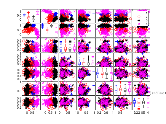
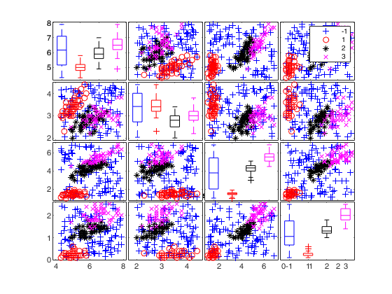
  • Add noise to an existing dataset.
  • Add outliers generated from uniform distribution to the IRIS dataset

    load fisheriris;
    Y=meas;
    Mu=grpstats(Y,species);
    S=zeros(4,4,3);
    S(:,:,1)=cov(Y(1:50,:));
    S(:,:,2)=cov(Y(51:100,:));
    S(:,:,3)=cov(Y(101:150,:));
    pigen=ones(3,1)/3;
    % Add 100 outliers and specify a very small value of alpha
    noisevars=0;
    noiseunits=struct;
    noiseunits.number=100;
    noiseunits.alpha=0.000001;
    % In this case the first argument which is supplied to simdataset is
    % the original matrix X
    [Ywithnoise,id]=simdataset(Y, pigen, Mu, S,'noisevars',noisevars,'noiseunits',noiseunits);
    spmplot(Ywithnoise,id,[],'box');
    title('4 groups with outliers from uniform')
    Click here for the graphical output of this example (link to Ro.S.A. website)

    Input Arguments

    expand all

    n — sample size or input matrix. Scalar.

    Scalar or matrix of size n-by-v. If n is a scalar it is interpreted as the sample size of the dataset which must be simulated. On the other hand, if n is a n-by-v it is interpreted as a matrix of size n-by-v which has to be contaminated with optional input arguments 'noiseunits' and 'noisevars'.

    Data Types: single| double

    Pi — Mixing proportions. Vector.

    Vector of size k containing mixing proportions. The sum of the elements of Pi is 1.

    Data Types: single| double

    Mu — centroids. Matrix.

    Matrix of size k-by-v containing (in the rows) the centroids of the k groups.

    Data Types: single| double

    S — Covariance matrices. 3D array.

    3D array of size v-by-v-by-k containing covariance matrices of the k groups.

    Data Types: single| double

    Name-Value Pair Arguments

    Specify optional comma-separated pairs of Name,Value arguments. Name is the argument name and Value is the corresponding value. Name must appear inside single quotes (' '). You can specify several name and value pair arguments in any order as Name1,Value1,...,NameN,ValueN.

    Example: 'noiseunits', 10 , 'noisevars', 5 , 'lambda',[1 1 0]; , 'R_seed',1;

    noiseunits —number of type of outlying observations.scalar | structure.

    Missing value, scalar or structure.

    This input parameter specifies the number and type of outlying observations. The default value of noiseunits is 0.

    - If noiseunits is a scalar t different from 0, then t units from the uniform distribution in the interval min(X) max(X) are generated in such a way that their squared Mahalanobis distance from the centroids of each existing group is larger then the quantile 1-0.999 of the Chi^2 distribution with p degrees of freedom. In order to generate these units the maximum number of attempts is equal to 10000.

    - If noiseunits is a structure it may contain the following fields: number = scalar, or vector of length f. The sum of the elements of vector 'number' is equal to the total number of outliers which are simulated.

    alpha = scalar or vector of legth f containing the level(s) of simulated outliers. The default value of alpha is 0.001.

    maxiter = maximum number of trials to simulate outliers.

    The default value of maxiter is 10000.

    interval= missing value or vector of length 2 or matrix of size 2-by-v which controls the min and max of the generated outliers for each dimension.

    If interval is empty (default), the outliers are simulated in the interval min(X) max(X).

    If interval is a vector of length(2), outliers for each variables are simulated in the range interval(1) and interval(2).

    If interval is a 2-by-v matrix outliers are simulated in: interval(1,1) interval (2,1) for variable 1 ...

    interval(1,v) interval (2,v) for variable v typeout = list of length f containing the type of outliers which must be simulated. Possible values for typeout are: * unif (or uniform), if the outliers must be generated using the uniform distribution;

    * norm (or normal), if the outliers must be generated using the normal distribution;

    * Chisquarez, if the outliers must be generated using the Chi2 distribution with z degrees of freedom;

    * Tz or tz, if the outliers must be generated using the Student T distribution with z degrees of freedom;

    * pointmass, if the outliers are concentrated on a particular point;

    * componentwise, if the outliers must have the same coordinates of the existing rows of matrix X apart from a single coordinate (which will be the min or max in that particular dimension or the min or max specified in interval).

    For example, the code: noiseunits=struct;

    Value Description
    number

    [100 100];

    typeout

    {'uniform' 'componentwise'};

    interval

    [-2 2];

    adds 200 outliers, the first 100 generated using a uniform distribution and the last 100 using componentwise scheme. Outliers are generated in the interval [-2 2] for each variable.

    Example: 'noiseunits', 10

    Data Types: double

    noisevars —Type of noise variables.scalar | structure.

    Empty value, scalar or structure.

    - If noisevars is not specified or is an empty value (default) no noise variable is added to the matrix of simulated data.

    - If noisevars is a scalar equal to r, then r new noise variables are added to the matrix of simulated data using the uniform distribution in the range [min(X) max(X)].

    - If noisevars is a structure it may contain the following fields:

    Value Description
    number

    a scalar or a vector of length f. The sum of elements of vector 'number' is equal to the total number of noise variables to be addded.

    distribution

    string or cell array of strings of length f which specifies the distribution to be used to simulate the noise variables.

    If field distribution is not present then the uniform distribution is used to simulate the noise variables.

    String 'distribution' can be one of the following values: * uniform = uniform distribution * normal = normal distribution * t or T followed by a number which controls the degrees of freedom. For example, t6 specifies to generate the data according to a Student T with 6 degrees of freedom.

    * chisquare followed by a number which controls the degreess of freedom. For example, chisquare8 specifies to generate the data according to a Chi square distribution with 8 degrees of freedom.

    interval

    string or vector of length 2 or matrix of size 2-by-f (where f is the number of noise variables) which controls for each element of vector 'number' or each element of cell 'distribution', the min and max of the noise variables. For example, interval(1,3) and interval(2,3) are respectively the minimum and maximum values of simulated the data for the third noise variable If interval is empty (default), the noise variables are simulated uniformly between the smallest and the largest coordinates of mean vectors.

    If interval is 'minmax' the noise varaibles are simulated uniformly between the smallest and the largest coordinates of the simulated data matrix.

    For example, the code: noisevars=struct;

    noisevars.number=[3 2];

    noisevars.distribution={'Chisquare5' 'T3'};

    noisevars.interval='minmax';

    adds 5 noise variables, the first 3 generated using the Chi2 with 5 degrees of freedom and the last two using the Student t with 3 degrees of freedom. Noise variables are generated in the interval min(X) max(X).

    Example: 'noisevars', 5

    Data Types: double

    lambda —Transformation coefficients.vector.

    Vector of length v containing inverse Box-Cox transformation coefficients. The value false (default) implies that no transformation is applied to any variable.

    Example: 'lambda',[1 1 0];

    Data Types: double

    R_seed —random numbers from R language.scalar.

    Scalar > 0 for the seed to be used to generate random numbers in a R instance. This is used to check consistency of the results obtained with the R package MixSim. See file Connect_Matlab_with_R_HELP to know how to connect MATLAB with R. This option requires the installation of the R-(D)COM Interface. Default is 0, i.e. random numbers are generated by matlab.

    Example: 'R_seed',1;

    Data Types: double

    Output Arguments

    expand all

    X —Simulated dataset. Matrix

    Simulated dataset of size (n + noiseunits)-by-(v + noisevars).

    Noise coordinates are provided in the last noisevars columns.

    id —Classification vector. Vector

    Classification vector of length n + noiseunits. Negative numbers represents the groups associated to the contaminated units.

    REMARK: If noiseunits outliers could not be generated a warning is produced. In this case matrix X and vector id will have less than n + noiseunits rows.

    References

    Maitra, R. and Melnykov, V. (2010), Simulating data to study performance of finite mixture modeling and clustering algorithms, "The Journal of Computational and Graphical Statistics", Vol. 19, pp. 354-376. [to refer to this publication we will use "MM2010 JCGS"]

    Melnykov, V., Chen, W.-C. and Maitra, R. (2012), MixSim: An R Package for Simulating Data to Study Performance of Clustering Algorithms, "Journal of Statistical Software", Vol. 51, pp. 1-25.

    Davies, R. (1980), The distribution of a linear combination of chi-square random variables, "Applied Statistics", Vol. 29, pp. 323-333.

    Riani, M., Cerioli, A., Perrotta, D. and Torti, F. (2015), Simulating mixtures of multivariate data with fixed cluster overlap in FSDA, "Advances in data analysis and classification", Vol. 9, pp. 461-481.

    https://doi.org/10.1007/s11634-015-0223-9

    This page has been automatically generated by our routine publishFS