FE_spot_vol_FFT
FE_spot_vol_FFT estimates the instantaneous variance of a diffusion process by the Fourier estimator with Dirichlet kernel, using the FFT algorithm
Syntax
Description
Examples
 Example of call of FE_spot_vol_FFT with just two input arguments.
Example of call of FE_spot_vol_FFT with just two input arguments.Generates price and instantaneous variance from the Constant Elasticity of Variance model [S. Beckers, The Journal of Finance, Vol. 35, No. 3, 1980] and estimates the instantaneous variance via the Fourier method.
n=1000;  T=1; t=0:T/n:T; S0=100;
[S,sigma]=CEVmodel(t,S0); % data generation
x=log(S); % log-price
spotvar=FE_spot_vol_FFT(x,t);
plot(spotvar(2:end-1))
ylabel('Spot variance')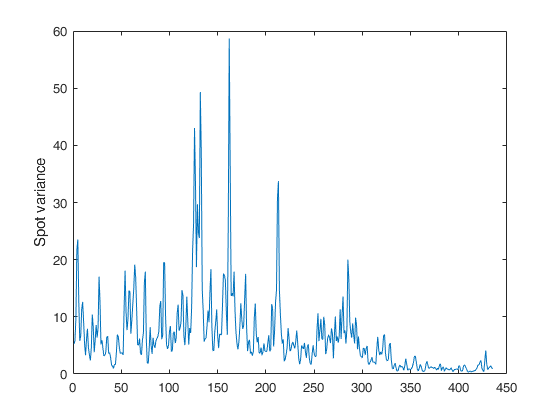
FE_spot_vol_FFT called with optional input argument N and M.
FE_spot_vol_FFT called with optional input argument N and M.Generates price and instantaneous variance from the Constant Elasticity of Variance model [S. Beckers, The Journal of Finance, Vol. 35, No. 3, 1980] and estimates the instantaneous variance via the Fourier method.
n=21600;  T=1; t=0:T/n:T; S0=100;
[S,sigma]=CEVmodel(t,S0); % data generation
x=log(S); % log-price
N=floor(n/2); M=floor(n^0.5); % cutting frequencies
spotvar=FE_spot_vol_FFT(x,t,'N',N,'M',M);
plot(spotvar(2:end-1))
ylabel('Spot variance')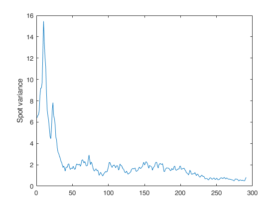
Example of call of FE_spot_vol_FFT providing both estimation values and times.
Example of call of FE_spot_vol_FFT providing both estimation values and times.Generates price and instantaneous variance from the Constant Elasticity of Variance model [S. Beckers, The Journal of Finance, Vol. 35, No. 3, 1980] and estimates the instantaneous variance via the Fourier method.
n=21600;  T=1; t=0:T/n:T; S0=100;
[S,sigma]=CEVmodel(t,S0); % data generation
x=log(S); % log-price
N=floor(n/2); M=150; % cutting frequencies
[spotvar,tau]=FE_spot_vol_FFT(x,t,'N',N,'M',M);
plot(tau,spotvar)
xlabel('time')
hold on; plot(tau,sigma(1:n/(2*M):end));
ylabel('Spot variance')
title('Estimated value (blue), True value (red)')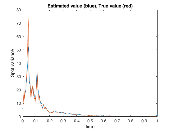
Input Arguments
Output Arguments
More About
References
Mancino, M.E., Recchioni, M.C., Sanfelici, S. (2017), Fourier-Malliavin Volatility Estimation. Theory and Practice, "Springer Briefs in Quantitative Finance", Springer.