FM_spot_volvol

FM_spot_volvol computes the spot volatiity of volatility of a diffusion process via the Fourier-Malliavin estimator

Syntax

  • VV_spot=FM_spot_volvol(x,t,T)example
  • VV_spot=FM_spot_volvol(x,t,T,Name,Value)example
  • [VV_spot, tau_out]=FM_spot_volvol(___)example

Description

example

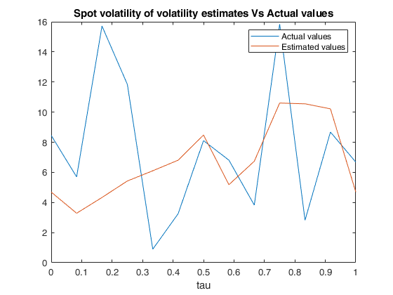
VV_spot =FM_spot_volvol(x, t, T) Example of call of FM_spot_volvol with default values of N,M,L and tau.
example

VV_spot =FM_spot_volvol(x, t, T, Name, Value) Example of call of FM_spot_volvol with custom choices of N,M,L and tau.

example

[VV_spot, tau_out] =FM_spot_volvol(___) Example of call of FM_spot_volvol when tau has length larger than 2L + 1.

Examples

expand all

  • Example of call of FM_spot_volvol with default values of N,M,L and tau.
  • The following example estimates the path of the spot volatility of volatility of a random process following the Heston model from a discrete sample. The Heston model assumes that the spot variance follows a Cox-Ingersoll-Ross model.

    % Heston model simulation
    T=1;  
    n=23400;  
    parameters=[0,0.8,10,3.25];
    rho=-0.3;
    x0=log(100); 
    V0=0.8;
    [x,V,t] = Heston1D(T,n,parameters,rho,x0,V0);
    % Spot volatility of volatility estimation  
    [VV_spot, tau_out] = FM_spot_volvol(x,t,T);
    L=(length(VV_spot)-1)/2;
    figure
    VV=parameters(end)^2*V;
    plot(tau_out,VV(1:round(n/(2*L)):end));
    hold on
    plot(tau_out,VV_spot); 
    xlabel('tau');
    title('Spot volatility of volatility estimates Vs Actual values')
    legend('Actual values','Estimated values')
    Click here for the graphical output of this example (link to Ro.S.A. website).

  • Example of call of FM_spot_volvol with custom choices of N,M,L and tau.
  • The following example estimates the daily path of the spot volatility of volatility of a random process following the Heston model from a discrete sample. The Heston model assumes that the spot variance follows a Cox-Ingersoll-Ross model.

    % Heston model simulation
    T=1; % horizon of the trajectory 
    n=23400; % number of observations simulated in one trajectory 
    parameters=[0,0.8,10,3.25];
    rho=-0.3;
    x0=log(100); 
    V0=0.8;
    [x,V,t]=Heston1D(T,n,parameters,rho,x0,V0);
    % Spot volatility of volatility estimation
    tau=0:T/10:T;
    [VV_spot, tau_out] = FM_spot_volvol(x,t,T,'N',10000,'M',50,'L',10,'tau',tau);
    figure
    VV=parameters(end)^2*V;
    plot(tau_out,VV(1:round(n/10):end));
    hold on
    plot(tau_out,VV_spot); 
    xlabel('tau'); 
    title('Spot volatility of volatility estimates Vs Actual values')
    legend('Actual values','Estimated values')
    Click here for the graphical output of this example (link to Ro.S.A. website).

  • Example of call of FM_spot_volvol when tau has length larger than 2L + 1.
  • The following example estimates the daily path of the spot volatility of volatility of a random process following the Heston model from a discrete sample. The Heston model assumes that the spot variance follows a Cox-Ingersoll-Ross model.

    % Heston model simulation
    T=1; % horizon of the trajectory 
    n=23400; % number of observations simulated in one trajectory 
    parameters=[0,0.8,10,3.25];
    rho=-0.3;
    x0=log(100); 
    V0=0.8;
    [x,V,t]=Heston1D(T,n,parameters,rho,x0,V0);
    % Spot volatility of volatility estimation
    tau=0:T/100:T;
    [VV_spot, tau_out] = FM_spot_volvol(x,t,T,'N',10000,'M',50,'L',10,'tau',tau);
    figure
    VV=parameters(end)^2*V;
    L=10;
    plot(tau_out,VV(1:round(n/(2*L)):end));
    hold on
    plot(tau_out,VV_spot); 
    xlabel('tau'); 
    title('Spot volatility of volatility estimates Vs Actual values')
    legend('Actual values','Estimated values')
    WARNING: estimation will be performed on the equally-spaced grid with mesh size equal to T/(2*L), provided as an output variable.
    
    Click here for the graphical output of this example (link to Ro.S.A. website).

    Input Arguments

    expand all

    x — Observed process values. Vector.

    Row or column vector containing the observed values.

    Data Types: single| double

    t — Observation times. Vector.

    Row or column vector with the same length of x containing the observation times.

    Data Types: single| double

    T — Estimation horizon. Scalar.

    Data Types: single| double

    Name-Value Pair Arguments

    Specify optional comma-separated pairs of Name,Value arguments. Name is the argument name and Value is the corresponding value. Name must appear inside single quotes (' '). You can specify several name and value pair arguments in any order as Name1,Value1,...,NameN,ValueN.

    Example: 'N',400 , 'M',20 , 'L',5 , 'tau', 0:T/100:T

    N —Cutting frequency.scalar.

    If N is not specified, it is set equal to floor((length(x)-1)/2).

    Example: 'N',400

    Data Types: single | double

    M —Cutting frequency.scalar.

    If M is not specified, it is set equal to floor(floor((length(x)-1)/2)^0.4).

    Example: 'M',20

    Data Types: single | double

    L —Cutting frequency.scalar.

    If L is not specified, it is set equal to floor(floor(floor((length(x)-1)/2)^0.4)^0.5).

    Example: 'L',5

    Data Types: single | double

    tau —Estimation times.vector.

    If tau is not specified, it is set equal to 0:T/(2*L):T.

    Example: 'tau', 0:T/100:T

    Data Types: single | double

    Output Arguments

    expand all

    VV_spot —Spot volatility of volatility estimates. Vector

    Estimated values of the spot volatility of volatility of the process.

    tau_out —Estimation times. Vector

    Coincides with the input vector tau unless the length of the latter is larger than 2L+1.

    More About

    expand all

    Additional Details

    We assume that the vectors x contains discrete observations from a diffusion process $x$ following the Ito stochastic differential equation $$dx(t)= \sigma(t) \ dW(t) + b(t) \ dt,$$ $$d\sigma^2(t)= \gamma(t) \ dZ(t) + a(t) \ dt,$$ where $W$ and $Z$ are two Brownian motions defined on the filtered probability space $(\Omega, (\mathcal{F}_t)_{t \in [0,T]}, P)$, with correlation $\rho$, while $\sigma, \gamma, b$ and $a$ are random processes, adapted to $\mathcal{F}_t$.

    See the References for further mathematical details.

    The spot volatility of volatility at time $t \in [0,T]$ is defined as $$C(t):=\frac{d\langle \sigma^2,\sigma^2 \rangle_t}{dt}=\gamma^2(t).$$ For any positive integer $n$, let $\mathcal{S}_{n}:=\{ 0=t_{0}\leq \cdots \leq t_{n}=T \}$ be the observation times. Moreover, let $\delta_l(x):= x(t_{l+1})-x(t_l)$ be the increments of $x$.

    The Fourier estimator of the spot volatility of volatility at time $t \in [0,T]$ is given by $$\widehat C_{n,N,M,L}(\tau)= \sum_{|k|\leq L} \left(1-{|k|\over L}\right)c_k(C_{n,N,M}) \, e^{{\rm i}\frac{2\pi}{T}k\tau},$$ where: $$c_k(C_{n,N,M})= {T \over {2M+1}} \sum_{|s|\leq M} c_s(d\sigma_{{n},N})c_{k-s}(d\sigma_{{n},N}),$$ $$c_k(d\sigma_{{n},N})={\rm i} \, k\, \frac{2\pi}{T} c_k(\sigma_{{n},N}), \quad c_k(\sigma_{n,N})={T\over {2N+1}} \sum_{|s|\leq N} c_{s}(dx_{n})c_{k-s}(dx_{n}),$$ $$c_k(dx_{n})= {1\over {T}} \sum_{l=0}^{n-1} e^{-{\rm i}\frac{2\pi}{T}kt_l}\delta_{l}(x).$$

    References

    Mancino, M.E., Recchioni, M.C., Sanfelici, S. (2017), Fourier-Malliavin Volatility Estimation. Theory and Practice, "Springer Briefs in Quantitative Finance", Springer.

    Sanfelici, S., Toscano, G. (2024), The Fourier-Malliavin Volatility (FMVol) MATLAB toolbox, available on ArXiv.

    This page has been automatically generated by our routine publishFS