FSRBr
Bayesian forward search in linear regression reweighted
Syntax
Description
FSRBr uses the units not declared as outliers by FSRB to produce a robust fit.
The units whose residuals exceeds the threshold determined by option alpha are declared as outliers. Moreover, it is possible in option R2th to modify the estimate of sigma2 which is used to declare the outliers. This is useful when there is almost a perfect fit in the data, the estimate of the error variance is very small and therefore there is the risk of declaring as outliers very small deviations from the robust fit. In this case, the estimate of sigma2 is corrected in order to achieve a value of R2 equal to R2th.
Example of FSRBr for international trade data (explore options).out
=FSRBr(y,
X,
Name, Value)
Examples
 Example of FSRBr for international trade data.
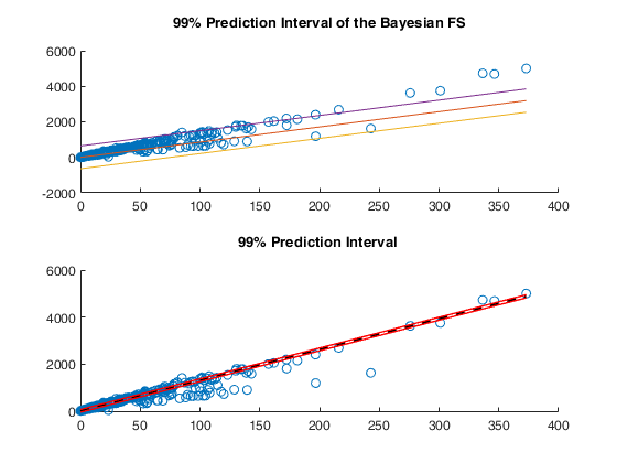
Example of FSRBr for international trade data.Bayesian FS to fit the group of undervalued flows.
load('fishery');
X = fishery{:,1};
y = fishery{:,2};
[n,p] = size(X);
X = X + 0.000001*randn(n,1);
% id = undervalued flows
id = (y./X < 9.5);
% my prior on beta
mybeta = median(y(id)./X(id));
bmad   = mad(y(id)./X(id));
ListIn = find(y./X <= mybeta + bmad);
% gscatter(X,y,id)
rr          = y(ListIn)-(X(ListIn,:) * mybeta);
numS2cl     = rr'*rr;
dfe         = length(ListIn)-p;
S2cl        = numS2cl/dfe;
bayes       = struct;
bayes.R     = X(ListIn,:)'*X(ListIn,:);
bayes.tau0  = 1/S2cl;
bayes.n0    = length(ListIn);
bayes.beta0 = mybeta;
% fit based on Bayesian FS with prior on the underdeclared flows
[out_B, xnew1 , ypred1, yci1]   = FSRBr(y,X,'bayes',bayes,'intercept',false,'alpha',0.01,'bonflev',0.999,'fullreweight',false,'plotsPI',1,'plots',0);
h1 = allchild(gca); a1 = gca; f1 = gcf;
% fit based on traditional FS
[out, xnew2 , ypred2, yci2]   = FSRr(y,X,'intercept',false,'alpha',0.01,'bonflev',0.999,'fullreweight',false,'plotsPI',1,'plots',0);
h2 = allchild(gca); a2 = gca; f2 = gcf;
% move the figure above into a single one with two panels
hh = figure; ax1 = subplot(2,1,1); ax2 = subplot(2,1,2);
copyobj(h1,ax1); title(ax1,get(get(a1,'title'),'string'));
copyobj(h2,ax2); title(ax2,get(get(a2,'title'),'string'));
figsize = get(hh, 'Position');
set(hh,'Position',figsize);
close(f1); close(f2);
disp(['Bayesian FS fit    = ' num2str(out_B.betar) ' using a prior based on undervalued flows']);
disp(['Traditional FS fit = ' num2str(out.betar)]);
Bayesian FS fit = 8.565 using a prior based on undervalued flows Traditional FS fit = 13.0939
Input Arguments
Output Arguments
References
Chaloner, K. and Brant, R. (1988), A Bayesian Approach to Outlier Detection and Residual Analysis, "Biometrika", Vol. 75, pp. 651-659.
Riani, M., Corbellini, A. and Atkinson, A.C. (2018), Very Robust Bayesian Regression for Fraud Detection, "International Statistical Review", http://dx.doi.org/10.1111/insr.12247
Atkinson, A.C., Corbellini, A. and Riani, M., (2017), Robust Bayesian Regression with the Forward Search: Theory and Data Analysis, "Test", Vol. 26, pp. 869-886, https://doi.org/10.1007/s11749-017-0542-6