ace

ace computes alternative conditional expectation

Syntax

Description

This function uses the alternating conditional expectation algorithm to find the transformations of y and X that maximise the proportion of variation in y explained by X. When X is a matrix, it is transformed so that its columns are equally weighted when predicting y.

example

out =ace(y, X) Example of the use of ace based on the Wang and Murphy data.

example

out =ace(y, X, Name, Value) Example 1 from TIB88: brain body weight data.

Examples

expand all

  • Example of the use of ace based on the Wang and Murphy data.
  • In order to have the possibility of replicating the results in R using library acepack function mtR is used to generate the random data.

    rng('default')
    seed=11;
    negstate=-30;
    n=200;
    X1 = mtR(n,0,seed)*2-1;
    X2 = mtR(n,0,negstate)*2-1;
    X3 = mtR(n,0,negstate)*2-1;
    X4 = mtR(n,0,negstate)*2-1;
    res=mtR(n,1,negstate);
    % Generate y
    y = log(4 + sin(3*X1) + abs(X2) + X3.^2 + X4 + .1*res );
    X = [X1 X2 X3 X4];
    % Apply the ace algorithm
    out= ace(y,X);
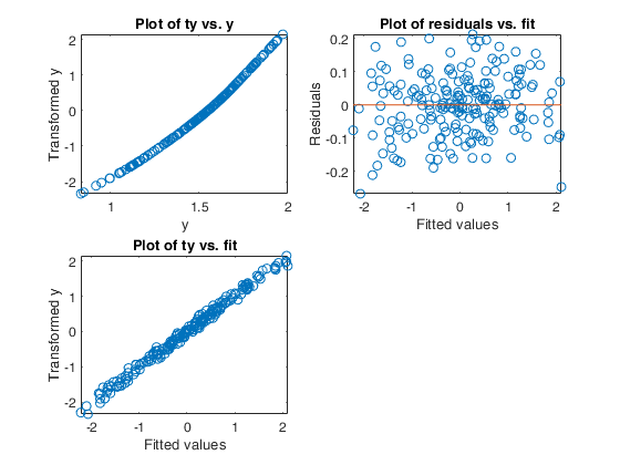
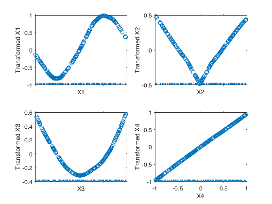
    % Show the output graphically using function aceplot
    aceplot(out)
    Click here for the graphical output of this example (link to Ro.S.A. website).

  • Example 1 from TIB88: brain body weight data.
  • Comparison between ace and avas.

    YY=load('animals.txt');
    y=YY(1:62,2);
    X=YY(1:62,1);
    out=ace(y,X);
    aceplot(out)
    out=avas(y,X);
    aceplot(out)
    % https://vincentarelbundock.github.io/Rdatasets/doc/robustbase/Animals2.html
    % ## The `same' plot for Rousseeuw's subset:
    % data(Animals, package = "MASS")
    % brain <- Animals[c(1:24, 26:25, 27:28),]
    % plotbb(bbdat = brain)

    Input Arguments

    expand all

    y — Response variable. Vector.

    Response variable, specified as a vector of length n, where n is the number of observations. Each entry in y is the response for the corresponding row of X.

    Missing values (NaN's) and infinite values (Inf's) are allowed, since observations (rows) with missing or infinite values will automatically be excluded from the computations.

    Data Types: single| double

    X — Predictor variables. Matrix.

    Matrix of explanatory variables (also called 'regressors') of dimension n x (p-1) where p denotes the number of explanatory variables including the intercept.

    Rows of X represent observations, and columns represent variables. By default, there is a constant term in the model, unless you explicitly remove it using input option intercept, so do not include a column of 1s in X. Missing values (NaN's) and infinite values (Inf's) are allowed, since observations (rows) with missing or infinite values will automatically be excluded from the computations.

    Data Types: single| double

    Name-Value Pair Arguments

    Specify optional comma-separated pairs of Name,Value arguments. Name is the argument name and Value is the corresponding value. Name must appear inside single quotes (' '). You can specify several name and value pair arguments in any order as Name1,Value1,...,NameN,ValueN.

    Example: 'l',[3 3 1] , 'w',1:n , 'nterm',5 , 'delrsq',0.001 , 'maxit',30

    l —type of transformation.vector.

    Vector of length p+1 which specifies how the type of transformation for the explanatory variables and the response. The first p element of this vector refers to the p explanatory variables, the last element refers to the response.

    l(j)=1 => j-th variable assumes orderable values.

    l(j)=2 => j-th variable assumes circular (periodic) values in the range (0.0,1.0) with period 1.0.

    l(j)=3 => j-th variable transformation is to be monotone.

    l(j)=4 => j-th variable transformation is to be linear.

    l(j)=5 => j-th variable assumes categorical (unorderable) values.

    j =1, 2, \ldots, p+1.

    The default value of l is a vector of ones of length p+1, this procedure assumes that both the explanatory variables and the response have orderable values.

    Example: 'l',[3 3 1]

    Data Types: double

    w —weights for the observations.vector.

    Row or column vector of length n containing the weights associated to each observations. If w is not specified we assume $w=1$ for $i=1, 2, \ldots, n$.

    Example: 'w',1:n

    Data Types: double

    nterm —minimum number of consecutive iteration below the threshold to terminate the outer loop.positive scalar.

    This value specifies how many consecutive iterations below the threshold it is necessary to have to declare convergence in the outer loop. The default value of nterm is 3.

    Example: 'nterm',5

    Data Types: double

    delrsq —termination threshold.scalar.

    Iteration (in the outer loop) stops when rsq changes less than delrsq in nterm. The default value of delrsq is 0.01.

    Example: 'delrsq',0.001

    Data Types: double

    maxit —maximum number of iterations for the outer loop.scalar.

    The default maximum number of iterations before exiting the outer loop is 20.

    Example: 'maxit',30

    Data Types: double

    Output Arguments

    expand all

    out — description Structure

    Structure which contains the following fields

    Value Description
    ty

    n x 1 vector containing the transformed y values.

    tX

    n x p matrix containing the transformed X matrix.

    rsq

    the multiple R-squared value for the transformed values in the last iteration of the outer loop.

    y

    n x 1 vector containing the original y values.

    X

    n x p matrix containing the original X matrix.

    niter

    scalar. Number of iterations which have been necessary to achieve convergence.

    outliers

    k x 1 vector containing the units declared as outliers when procedure is called with input option rob set to true. If rob is false out.outliers=[].

    References

    Breiman, L. and Friedman, J.H. (1985), Estimating optimal transformations for multiple regression and correlation, "Journal of the American Statistical Association", Vol. 80, pp. 580-597.

    Wang D. and Murphy M. (2005), Identifying nonlinear relationships regression using the ACE algorithm, "Journal of Applied Statistics", Vol. 32, pp. 243-258.

    This page has been automatically generated by our routine publishFS