aceplot
aceplot produces the aceplot to visualize the results of ace
Description
This function produces two figures. The first figure contains: the plot of transformed y vs. y (top left panel), the plot of residuals vs. fit (top right panel) and the plot of transformed y vs. fit (bottom left panel). The bottom right panel is left blank. This first figure is tagged pl_ty.
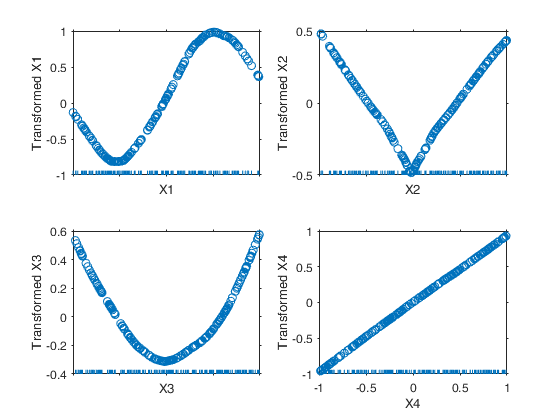
The second figure contains a series of p panels (where p is the number of columns of X) for transformed $X_j$ (tXj) vs. $X_j$ (with a rug plot along the tick marks). The second figure is tagged pl_tX.
These two figures can be combined in one figure, putting the plots of tXj vs $X_j$ in the bottom right panel of the first figure using optional input argument oneplot. If just one figure is produced it is tagged pl_tyX.
aceplot(
Example of use of option highlight.out,
Name, Value)
Examples
 Example of the use of ace based on the Wang and Murphy data.
Example of the use of ace based on the Wang and Murphy data.In order to have the possibility of replicating the results in R using library acepack function mtR is used to generate the random data.
rng('default')
seed=11;
negstate=-30;
n=200;
X1 = mtR(n,0,seed)*2-1;
X2 = mtR(n,0,negstate)*2-1;
X3 = mtR(n,0,negstate)*2-1;
X4 = mtR(n,0,negstate)*2-1;
res=mtR(n,1,negstate);
% Generate y
y = log(4 + sin(3*X1) + abs(X2) + X3.^2 + X4 + .1*res );
X = [X1 X2 X3 X4];
% Apply the ace algorithm
out= ace(y,X);
% Show the output graphically using function aceplot
aceplot(out)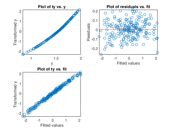
Related Examples
Input Arguments
Output Arguments
References
Breiman, L. and Friedman, J.H. (1985), Estimating optimal transformations for multiple regression and correlation, "Journal of the American Statistical Association", Vol. 80, pp. 580-597.
Wang D. and Murphy M. (2005), Identifying nonlinear relationships regression using the ACE algorithm, "Journal of Applied Statistics", Vol. 32, pp. 243-258.