avasmsplot
avasmsplot produces the augmented star plot and enables interactivity
Description
Examples
 Example from Wang and Murphy: avasmsplot with all default options.
Example from Wang and Murphy: avasmsplot with all default options.
close all
rng('default')
seed=100;
negstate=-30;
n=200;
X1 = mtR(n,0,seed)*2-1;
X2 = mtR(n,0,negstate)*2-1;
X3 = mtR(n,0,negstate)*2-1;
X4 = mtR(n,0,negstate)*2-1;
res=mtR(n,1,negstate);
% Generate y
y = log(4 + sin(3*X1) + abs(X2) + X3.^2 + X4 + .1*res );
X = [X1 X2 X3 X4];
y([121 80 34 188 137 110 79 86 1])=1.9+randn(9,1)*0.01;
% Automatic model selection
[VALtfin,Resarraychk]=avasms(y,X,'plots',0);
% Show the best solutions
avasmsplot(VALtfin);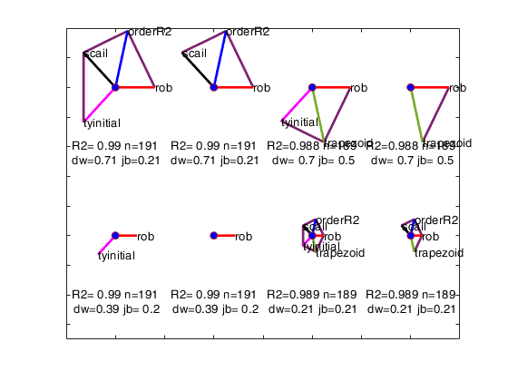
Example of option maxBestSol.
Example of option maxBestSol.
close all
% Example from Wang and Murphy:
rng('default')
seed=100;
negstate=-30;
n=200;
X1 = mtR(n,0,seed)*2-1;
X2 = mtR(n,0,negstate)*2-1;
X3 = mtR(n,0,negstate)*2-1;
X4 = mtR(n,0,negstate)*2-1;
res=mtR(n,1,negstate);
% Generate y
y = log(4 + sin(3*X1) + abs(X2) + X3.^2 + X4 + .1*res );
X = [X1 X2 X3 X4];
y([121 80 34 188 137 110 79 86 1])=1.9+randn(9,1)*0.01;
% Automatic model selection
[VALtfin,Resarraychk]=avasms(y,X,'plots',0);
% Show just the 4 best solutions
avasmsplot(VALtfin,'maxBestSol',4);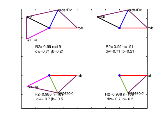
Related Examples
Input Arguments
Output Arguments
References
Riani M. and Atkinson A.C. and Corbellini A. (2023), Robust Transformations for Multiple Regression via Additivity and Variance Stabilization, submitted.