avasms
avasms computes avas using a series of alternative options
Syntax
Description
This function applies avas with a series of options and produces the augmented star plot.
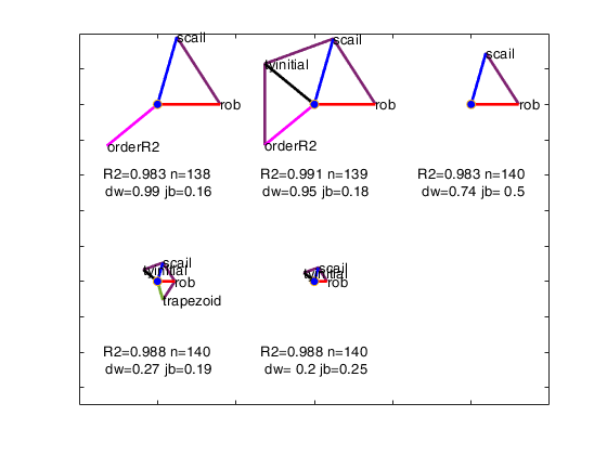
Below we list the five options giving an informative text description followed by the optional input arguments. We also give in parenthesis, the abbreviations used in the augmented star plot, where these are different.
- Robustness (rob).
- Remove effect of order of explanatory variables by regression (scail).
- Trapezoidal or rectangular rule for numerical integration in function ctsub (trapezoid).
- Ordering inclusion of the variables in the backfitting algorithm using values (orderR2).
- Initial robust transformation of the response (tyinitial).
We reduce the number of analyses for investigation by removing all those for which the residuals fail the Durbin-Watson and Jarque-Bera tests, at the 10 per cent level (two-sided for Durbin-Watson). Unlike the Durbin-Watson test, the Jarque-Bera test uses a combination of estimated skewness and kurtosis to test for distributional shape of the residuals.
Note that this threshold of 10 per cent can be changed using optional input argument critBestSol.
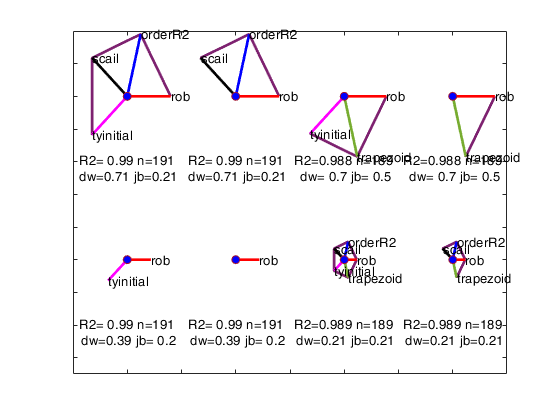
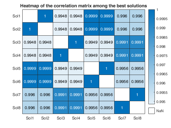
We order the solutions by the Durbin-Watson significance level multiplied by the value of R^2 and by the number of units not declared as outliers. The rays in individual plots are of equal length for those features used in an analysis. All rays are in identical places in each plot. Information in the plot is augmented by making the length of the rays for each analysis reflect the properties of the analysis; they are proportional to p_{DW}, the significance level of the Durbin-Watson test. Note that the ordering in which the solutions are displayed in the plot can be changed using optional input argument SolutionOrdering.
The five options start on the right and wind counterclockwise in steps of 72 degrees around the circle. The ordering in which the five options are displayed in the plot depends on the frequency of presence among the set of the admissible solutions. For example, if robustness is the one who has the highest frequency, its spoke is shown on the right (plotted to the East). The second most present option is shown on the top right...
and the least present option is shown on the bottom right.
Wang and Murphy data.BestSol
=avasms(y,
X,
Name, Value)
Examples
 Example 2 in RAC (2022).
Example 2 in RAC (2022).There are four explanatory variables and 151 observations with x_1 equally spaced from 0:0.1:15. The linear model is: z = \text{sin}(x) + \sum_{j=2}^4 (j-1)x_j + 0.5\mathcal{U}(-0.5,0.5), where x_{ij} (j=2, \ldots, 4), are independently \mathcal{N}(0,1). Eight outliers of value one replace the values of z at x = 8.9, 9.9, 10.4, 10.5 ... 10.9. The response y = \exp z. There are thus four explanatory variables, only one of which requires transformation, as does the response to logy.
rng(100)
x1 = (0:0.1:15)';
n=length(x1);
X3=randn(n,3);
Xb=X3*(1:3)';
z = sin(x1) + 0.5*(rand(size(x1))-0.5)+Xb;
z([90,100,105:110]) = 1;
X=[x1 X3];
y=exp(z);
% Automatic model selection
[BestSol,corMatrix]=avasms(y,X);
No model found with pvalDW>0.1 and pvalJB>0.1
Setting pvalDW=0.05 and pvalJB=0.05
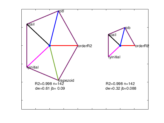
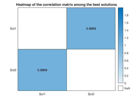
Wang and Murphy data.
Wang and Murphy data.
rng('default')
seed=100;
negstate=-30;
n=200;
X1 = mtR(n,0,seed)*2-1;
X2 = mtR(n,0,negstate)*2-1;
X3 = mtR(n,0,negstate)*2-1;
X4 = mtR(n,0,negstate)*2-1;
res=mtR(n,1,negstate);
% Generate y
y = log(4 + sin(3*X1) + abs(X2) + X3.^2 + X4 + .1*res );
X = [X1 X2 X3 X4];
y([121 80 34 188 137 110 79 86 1])=1.9+randn(9,1)*0.01;
[BestSol,corMatrix]=avasms(y,X);

Example of the use of avasms using the Fish data.
Example of the use of avasms using the Fish data.
load("fish.mat");
Y=fish;
% pike is removed. We use just the first 3 explanatory variables.
sel=categorical(Y{:,1})~='Pike';
y=Y{sel,2};
X=Y{sel,3:5};
[BestSol,corMatrix]=avasms(y,X,'l',3*ones(size(X,2),1));

Related Examples
Input Arguments
Output Arguments
More About
References
Riani M., Atkinson A.C. and Corbellini A. (2022), Robust Transformations for Multiple Regression via Additivity and Variance Stabilization, submitted.
Tibshirani R. (1987), Estimating optimal transformations for regression, "Journal of the American Statistical Association", Vol. 83, 394-405.
Wang D. and Murphy M. (2005), Identifying nonlinear relationships regression using the ACE algorithm, "Journal of Applied Statistics", Vol. 32, pp. 243-258.