avas
avas computes additivity and variance stabilization for regression
Description
Examples
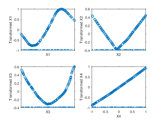
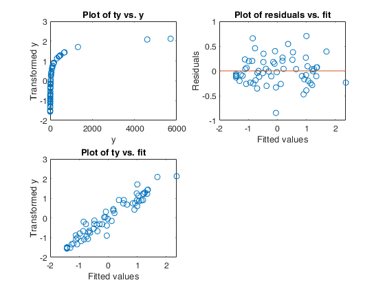
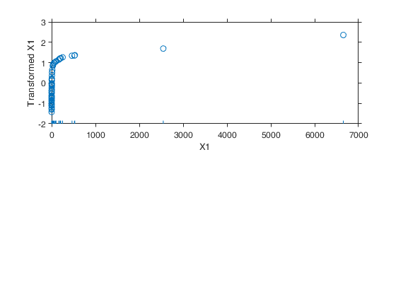
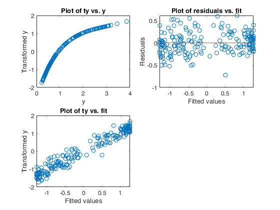
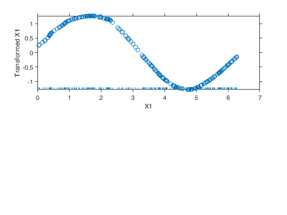
 Example of the use of avas based on the Wang and Murphy data.
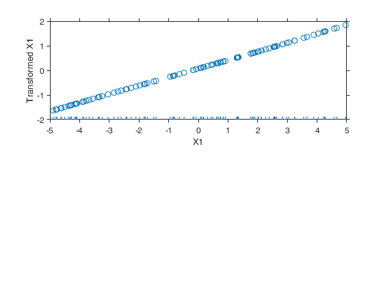
Example of the use of avas based on the Wang and Murphy data.In order to have the possibility of replicating the results in R using library acepack function mtR is used to generate the random data.
rng('default')
seed=11;
negstate=-30;
n=200;
X1 = mtR(n,0,seed)*2-1;
X2 = mtR(n,0,negstate)*2-1;
X3 = mtR(n,0,negstate)*2-1;
X4 = mtR(n,0,negstate)*2-1;
res=mtR(n,1,negstate);
% Generate y
y = log(4 + sin(3*X1) + abs(X2) + X3.^2 + X4 + .1*res );
X = [X1 X2 X3 X4];
% Apply the avas algorithm
out= avas(y,X);
% Show the output graphically using function aceplot
aceplot(out)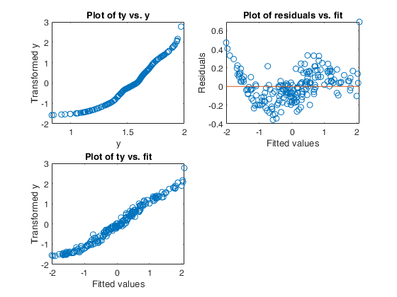
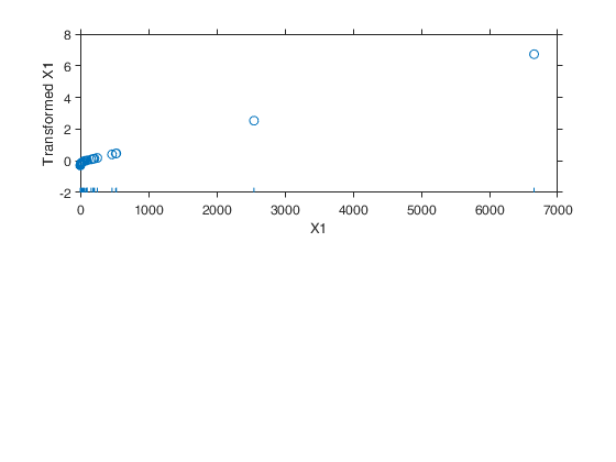
Example 1 from TIB88: brain body weight data.
Example 1 from TIB88: brain body weight data.Comparison between ace and avas.
YY=load('animals.txt');
y=YY(1:62,2);
X=YY(1:62,1);
out=ace(y,X);
aceplot(out)
out=avas(y,X);
aceplot(out)
% https://vincentarelbundock.github.io/Rdatasets/doc/robustbase/Animals2.html
% ## The `same' plot for Rousseeuw's subset:
% data(Animals, package = "MASS")
% brain <- Animals[c(1:24, 26:25, 27:28),]
% plotbb(bbdat = brain)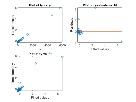
Related Examples
Example 3 from TIB88: unequal variances.
Example 3 from TIB88: unequal variances.
n=200;
rng('default')
seed=100;
negstate=-30;
x = mtR(n,0,seed)*3;
z = mtR(n,1,negstate);
y=x+0.1*x.*z;
X=x;
nr=1;
nc=2;
outACE=ace(y,X);
outAVAS=avas(y,X);
subplot(nr,nc,1)
yy=[y, outACE.ty outAVAS.ty];
yysor=sortrows(yy,1);
plot(yysor(:,1),yysor(:,2:3))
% plot(y,[outACE.ty outAVAS.ty])
title('Compare ACE and AVAS')
xlabel('y')
ylabel('ty')
legend({'ACE' 'AVAS'},'Location','Best')
subplot(nr,nc,2)
XX=[X, outACE.tX outAVAS.tX];
XXsor=sortrows(XX,1);
plot(XXsor(:,1),XXsor(:,2:3))
% plot(y,[outACE.ty outAVAS.ty])
title('Compare ACE and AVAS')
xlabel('x')
ylabel('tX')
legend({'ACE' 'AVAS'},'Location','Best')
% For R users, the R code to reproduce the example above is given
% below.
% set.seed(100)
% n=200
% x <- runif(n)*3
% z <- rnorm(n)
% y=x+0.1*x*z;
% out=ace(x,y)
% out=avas(x,y)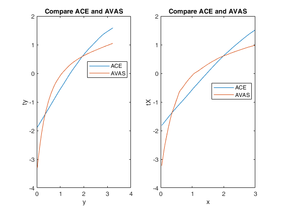
Example 4 from TIB88: non constant underlying variance.
Example 4 from TIB88: non constant underlying variance.
close all
negstate=-100;
rng('default')
seed=100;
n=200;
x1=mtR(n,1,seed);
x2=mtR(n,1,negstate);
z=mtR(n,1,negstate);
% x1=randn(n,1);
% x2=randn(n,1);
% z=randn(n,1);
absx1_x2=abs(x1-x2);
y=x1+x2+(1/3)*absx1_x2.*z;
X=[x1 x2];
out=avas(y,X);
tyhat=sum(out.tX,2);
ty=out.ty;
absty_tyhat=abs(ty-tyhat);
% hold('on')
plot(absx1_x2,absty_tyhat,'o');
lsline
% For R users, the R code to reproduce the example above is given
% below.
% # Example 4 non constant underlying variance
%  set.seed(100)
% n=200;
% x1=rnorm(n);
% x2=rnorm(n);
% z=rnorm(n);
% absx1_x2=abs(x1-x2);
% y=x1+x2+(1/3)*absx1_x2*z;
% X=cbind(x1,x2);
% out=avas(X,y);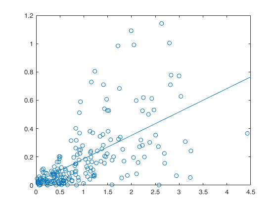
Example 5 from TIB88: missing group variable.
Example 5 from TIB88: missing group variable.
rng('default')
seed=1000;
n=100;
x=mtR(n,0,seed)*10-5;
z=mtR(n,1,-seed);
%x=rand(n,1)*10-5;
%z=randn(n,1);
y1=3+5*x+z;
y2=-3+5*x+z;
y=[y1;y2];
X=[x;x];
out=avas(y,X);
aceplot(out);
% For R users, the R code to reproduce the example above is given
% below.
% # Example 5 missing group variable
% set.seed(1000)
% n=100;
% x=runif(n)*10-5;
% z=rnorm(n);
% y1=3+5*x+z;
% y2=-3+5*x+z;
% y=c(y1,y2);
% X=c(x,x)
% out=avas(X,y);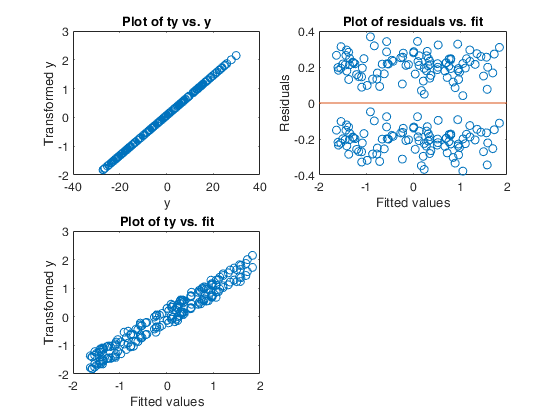
Example 6 from TIB88: binary.
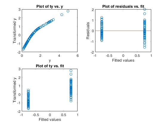
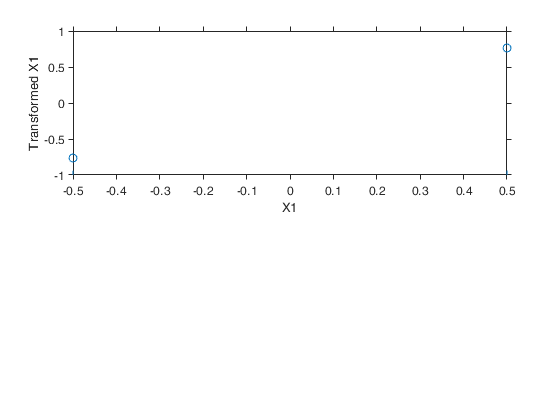
Example 6 from TIB88: binary.
seed=20;
n=50;
y1=exp(-0.5+0.5*mtR(n,1,seed));
y2=exp(0.5+0.5*mtR(n,1,-seed));
y=[y1;y2];
X=[-0.5*ones(n,1); 0.5*ones(n,1)];
out=avas(y,X);
aceplot(out)
% For R users, the R code to reproduce the example above is given
% below.
% Example 6 binary
% set.seed(20)
% n=50;
% y1=exp(-0.5+0.5*rnorm(n));
% y2=exp(0.5+0.5*rnorm(n));
% y=c(y1,y2);
% X=c(-0.5*rep(1,n), 0.5*rep(1,n));
% out=avas(X,y);
Example 9 from TIB88: Nonmonotone function of X.
Example 9 from TIB88: Nonmonotone function of X.
n=200;
x=rand(n,1)*2*pi;
z=randn(n,1);
y=exp(sin(x)+0.2*z);
X=x;
out=avas(y,X);
aceplot(out)
Input Arguments
Output Arguments
More About
References
Tibshirani R. (1987), Estimating optimal transformations for regression, "Journal of the American Statistical Association", Vol. 83, 394-405.
Wang D. and Murphy M. (2005), Identifying nonlinear relationships regression using the ACE algorithm, "Journal of Applied Statistics", Vol. 32, pp. 243-258.