overlapmap
overlapmap produces an interactive overlap map
Description
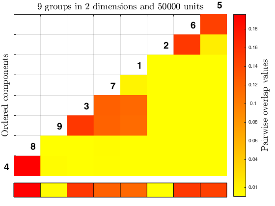
The function overlapmap plots the ordered pairwise overlap values between components. These components are ordered according to a specific rule:
first the closest pair is plotted in the lowest left corner, then the components closer to the ones already included are plotted (when all of them have a zero overlap value with the ones already included, the closest pair between all the remaining ones is inserted). The overlap map can either shows with different colors the closeness between components (i.e. in a descriptive manner), or it becomes an interactive plot with a left click on the color bar, which find and visualize the closest components according to a specific threshold value $ \omega^* $ (i.e. omegaStar), which specifies the minimum pairwise overlap threshold value used to merge the components. The interactive process ends with a right click on the white grid in the upper left corner of the plot, it also updates the results creating in the workspace a new variable 'userOverlap'. See the More About section for further information.
Example using M5data with tclust and tkmeans, specifying an
initial threshold omegaStar, a colormap, and allowing for additional
interactive plots.out
=overlapmap(D,
Name, Value)
Examples
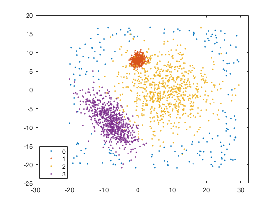
 Example using tkmeans on geyser data.
Example using tkmeans on geyser data.
close all
Y = load('geyser2.txt');
k = 3;
% using tkmeans
out = tkmeans(Y, k*2, 0.05, 'plots', 1);
overl_1 = overlapmap(out);
% using tkmeans for a higher number of components
out2 = tkmeans(Y, k*4, 0.05, 'plots', 1);
overl_2 = overlapmap(out2);
Total estimated time to complete trimmed k means: 0.14 seconds Total estimated time to complete trimmed k means: 0.34 seconds
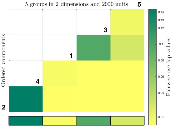
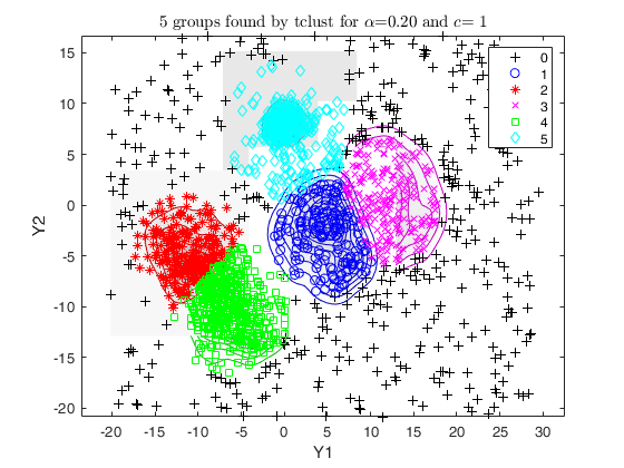
Example using M5data with tclust and tkmeans, specifying an
initial threshold omegaStar, a colormap, and allowing for additional
interactive plots.
Example using M5data with tclust and tkmeans, specifying an
initial threshold omegaStar, a colormap, and allowing for additional
interactive plots.
close all
rng('default')
rng(2)
Y=load('M5data.txt');
gscatter(Y(:,1),Y(:,2), Y(:,3))
k = 3;
out = tkmeans(Y(:,1:2), k*5, 0.2, 'plots', 'ellipse', 'Ysave', true);
overl = overlapmap(out, 'omegaStar', 0.025, 'plots', 'contour', 'userColors', winter);
rng('default')
if verLessThan('matlab', '8.5')
rng(5)
else
rng(1)
end
out_2 = tclust(Y(:,1:2), k*2, 0.2, 1, 'plots', 'contourf', 'Ysave', true);
overl_2 = overlapmap(out_2, 'omegaStar', 0.0025, 'plots', 'contourf', 'userColors', summer);
Total estimated time to complete trimmed k means: 2.69 seconds ------------------------------ Warning: Number of subsets without convergence equal to 36% ClaLik with untrimmed units selected using crisp criterion Total estimated time to complete tclust: 3.36 seconds Number of supplied clusters =6 Number of estimated clusters =5 Warning: The total number of estimated clusters is smaller than the number supplied
Related Examples
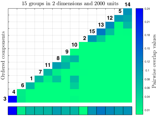
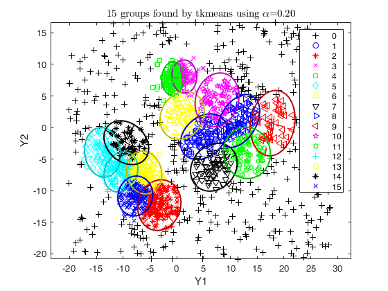
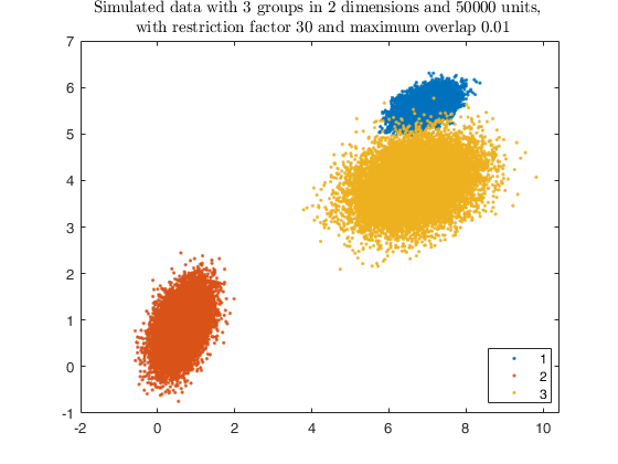
Example using simdataset to create heterogeneous and elliptical
clusters and using tkmeans output as input for the overlap map.
Example using simdataset to create heterogeneous and elliptical
clusters and using tkmeans output as input for the overlap map.
close all
% Specify k cluster in v dimensions with n obs
k = 3;
v = 2;
n = 50000;
% restriction factor
restr = 30;
% Maximum overlap
maxOm = 0.005;
% Generate heterogeneous and elliptical clusters
rng('default')
rng(500, 'twister');
out = MixSim(k, v, 'sph', false, 'restrfactor', restr, 'int', [0 10], ...
'Display', 'off', 'MaxOmega', maxOm, 'Display','off');
% null noise
alpha0 = 0;
% Simulating data
[X, id] = simdataset(n, out.Pi, out.Mu, out.S, 'noiseunits', alpha0);
% Plotting data
gg = gscatter(X(:,1), X(:,2), id);
str = sprintf('Simulated data with %d groups in %d dimensions and %d units, \n with restriction factor %d and maximum overlap %.2f', ...
k, v, n, restr, maxOm);
title(str,'Interpreter','Latex');
% use tkmeans for a larger number of cluster and without trimming
tkm = tkmeans(X, k*3, 0,'plots', 2,'Ysave',true, 'plots', 'ellipse');
% overlap map with interctive mode
overl = overlapmap(tkm, 'omegaStar', 0.01, 'plots', 'contourf');
Total estimated time to complete trimmed k means: 32.17 seconds ------------------------------ Warning: Number of subsets without convergence equal to 37.3333%
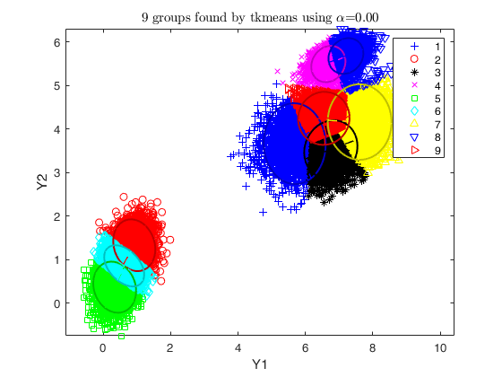
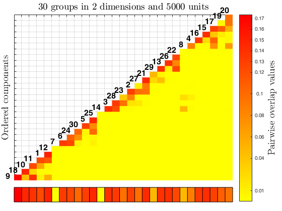
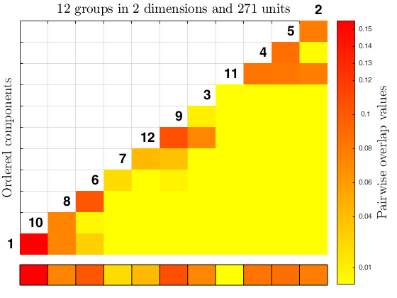
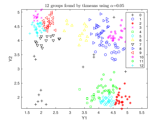
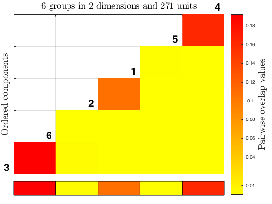
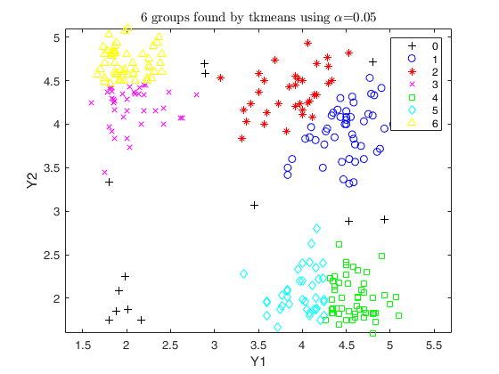
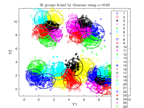
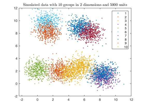
Example using simdataset to create homogeneous and spherical clusters
and using tkmeans.
Example using simdataset to create homogeneous and spherical clusters
and using tkmeans.
clear variables; close all
% Specify k cluster in v dimensions with n obs
k = 10;
v = 2;
n = 5000;
% Generate homogeneous and spherical clusters
rng('default')
rng(100, 'twister');
out = MixSim(k, v, 'sph', true, 'hom', true, 'int', [0 10], 'Display', 'off', 'BarOmega', 0.05, 'Display','off');
% Simulating data
[X, id] = simdataset(n, out.Pi, out.Mu, out.S);
% Plotting data
gscatter(X(:,1), X(:,2), id);
str = sprintf('Simulated data with %d groups in %d dimensions and %d units', k, v, n);
title(str,'Interpreter','Latex');
clickableMultiLegend(num2str((1:k)'));
% use tkmeans for a larger number of cluster and without trimming
tkm = tkmeans(X, k*3, 0,'plots', 2,'Ysave',true, 'plots', 'ellipse');
% overlap map with interctive mode
out = overlapmap(tkm, 'omegaStar', 0.01, 'plots', 'contourf');
Total estimated time to complete trimmed k means: 17.75 seconds ------------------------------ Warning: Number of subsets without convergence equal to 36%

Input Arguments
Output Arguments
More About
References
Melnykov, V., Michael, S. (2020), Clustering Large Datasets by Merging K-Means Solutions, Journal of Classification, Vol. 37, pp. 97–123, https://doi.org/10.1007/s00357-019-09314-8
Melnykov, V. (2016), Merging Mixture Components for Clustering Through Pairwise Overlap, "Journal of Computational and Graphical Statistics", Vol. 25, pp. 66-90.
Acknowledgements
...