
|
ASrho |
avas |
 |
ASwei
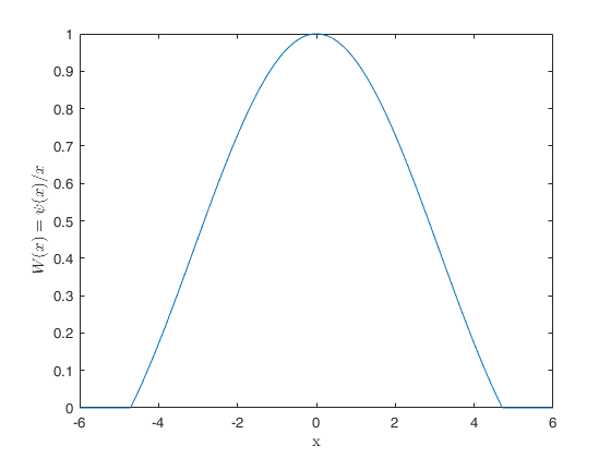
ASwei computes weight function psi(u)/u for Andrew's sine function
Syntax
weiAS=ASwei(u,c)example
Examples
 Weight function for Andrew's sine link.
Weight function for Andrew's sine link.
x=-6:0.01:6;
c=1.5;
weiAS=ASwei(x,c);
plot(x,weiAS)
xlabel('x','Interpreter','Latex')
ylabel('$W (x) =\psi(x)/x$','Interpreter','Latex')
Related Examples
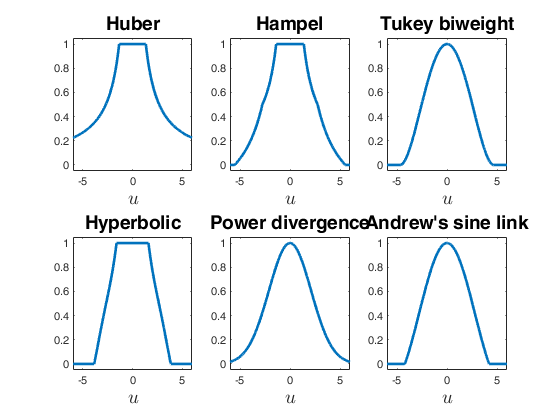
Compare six different weight functions in each of them eff is 95 per cent.
Compare six different weight functions in each of them eff is 95 per cent.Initialize graphical parameters.
FontSize=14;
x=-6:0.01:6;
ylim1=-0.05;
ylim2=1.05;
xlim1=min(x);
xlim2=max(x);
LineWidth=2;
subplot(2,3,1)
ceff095HU=HUeff(0.95,1);
weiHU=HUwei(x,ceff095HU);
plot(x,weiHU,'LineWidth',LineWidth)
xlabel('$u$','Interpreter','Latex','FontSize',FontSize)
title('Huber','FontSize',FontSize)
ylim([ylim1 ylim2])
xlim([xlim1 xlim2])
subplot(2,3,2)
ceff095HA=HAeff(0.95,1);
weiHA=HAwei(x,ceff095HA);
plot(x,weiHA,'LineWidth',LineWidth)
xlabel('$u$','Interpreter','Latex','FontSize',FontSize)
title('Hampel','FontSize',FontSize)
ylim([ylim1 ylim2])
xlim([xlim1 xlim2])
subplot(2,3,3)
ceff095TB=TBeff(0.95,1);
weiTB=TBwei(x,ceff095TB);
plot(x,weiTB,'LineWidth',LineWidth)
xlabel('$u$','Interpreter','Latex','FontSize',FontSize)
title('Tukey biweight','FontSize',FontSize)
ylim([ylim1 ylim2])
xlim([xlim1 xlim2])
subplot(2,3,4)
ceff095HYP=HYPeff(0.95,1);
ktuning=4.5;
weiHYP=HYPwei(x,[ceff095HYP,ktuning]);
plot(x,weiHYP,'LineWidth',LineWidth)
xlabel('$u$','Interpreter','Latex','FontSize',FontSize)
title('Hyperbolic','FontSize',FontSize)
ylim([ylim1 ylim2])
xlim([xlim1 xlim2])
subplot(2,3,5)
ceff095PD=PDeff(0.95);
weiPD=PDwei(x,ceff095PD);
weiPD=weiPD/max(weiPD);
plot(x,weiPD,'LineWidth',LineWidth)
xlabel('$u$','Interpreter','Latex','FontSize',FontSize)
title('Power divergence','FontSize',FontSize)
ylim([ylim1 ylim2])
xlim([xlim1 xlim2])
subplot(2,3,6)
ceff095AS=ASeff(0.95);
weiAS=ASwei(x,ceff095AS);
weiAS=weiAS/max(weiAS);
plot(x,weiAS,'LineWidth',LineWidth)
xlabel('$u$','Interpreter','Latex','FontSize',FontSize)
title('Andrew''s sine link','FontSize',FontSize)
ylim([ylim1 ylim2])
xlim([xlim1 xlim2])
Input Arguments
Output Arguments
More About
References
Andrews, D.F., Bickel, P.J., Hampel, F.R., Huber, P.J., Rogers, W.H., and Tukey, J.W. (1972), "Robust Estimates of Location: Survey and Advances", Princeton Univ. Press, Princeton, NJ. [p. 203]
Andrews, D. F. (1974). A Robust Method for Multiple Linear Regression, "Technometrics", V. 16, pp. 523-531, https://doi.org/10.1080/00401706.1974.10489233
|
|
ASrho |
avas |
|
|
|
Functions |
|
• The developers of the toolbox • The forward search group • Terms of Use • Acknowledgments