
|
FSRts |
FSRtsmdr |
 |
FSRtsbsb
FSRtsbsb returns the units belonging to the subset in each step of the forward search
Description
Examples
 FSRtsbsb with optional arguments.
FSRtsbsb with optional arguments.Load airline data 1949 1950 1951 1952 1953 1954 1955 1956 1957 1958 1959 1960.
y = [112 115 145 171 196 204 242 284 315 340 360 417 % Jan
118 126 150 180 196 188 233 277 301 318 342 391 % Feb
132 141 178 193 236 235 267 317 356 362 406 419 % Mar
129 135 163 181 235 227 269 313 348 348 396 461 % Apr
121 125 172 183 229 234 270 318 355 363 420 472 % May
135 149 178 218 243 264 315 374 422 435 472 535 % Jun
148 170 199 230 264 302 364 413 465 491 548 622 % Jul
148 170 199 242 272 293 347 405 467 505 559 606 % Aug
136 158 184 209 237 259 312 355 404 404 463 508 % Sep
119 133 162 191 211 229 274 306 347 359 407 461 % Oct
104 114 146 172 180 203 237 271 305 310 362 390 % Nov
118 140 166 194 201 229 278 306 336 337 405 432 ]; % Dec
y=(y(:));
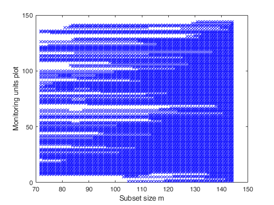
% Define the model and show the monitoring units plots.
model=struct;
model.trend=1; % linear trend
model.s=12; % monthly time series
model.seasonal=104; % four harmonics with time varying seasonality
bsbini=[97 77 12 2 26 95 10 60 94 135 7 61 114];
[Un,BB]=FSRtsbsb(y,bsbini,'model',model,'plots',1);

Monitoring the units belonging to subset.
Monitoring the units belonging to subset.Load airline data.
% 1949 1950 1951 1952 1953 1954 1955 1956 1957 1958 1959 1960
y = [112 115 145 171 196 204 242 284 315 340 360 417 % Jan
118 126 150 180 196 188 233 277 301 318 342 391 % Feb
132 141 178 193 236 235 267 317 356 362 406 419 % Mar
129 135 163 181 235 227 269 313 348 348 396 461 % Apr
121 125 172 183 229 234 270 318 355 363 420 472 % May
135 149 178 218 243 264 315 374 422 435 472 535 % Jun
148 170 199 230 264 302 364 413 465 491 548 622 % Jul
148 170 199 242 272 293 347 405 467 505 559 606 % Aug
136 158 184 209 237 259 312 355 404 404 463 508 % Sep
119 133 162 191 211 229 274 306 347 359 407 461 % Oct
104 114 146 172 180 203 237 271 305 310 362 390 % Nov
118 140 166 194 201 229 278 306 336 337 405 432 ]; % Dec
y=(y(:));
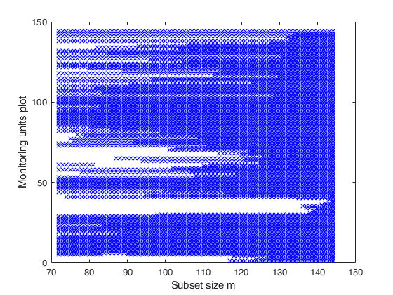
% Contaminates units 31:40
y(31:40)=y(31:40)+200;
% Define the model and show the monitoring units plots.
model=struct;
model.trend=1; % linear trend
model.s=12; % monthly time series
model.seasonal=104; % four harmonics with time varying seasonality
bsbini=[97 77 12 2 26 95 10 60 94 135 7 61 114];
[Un,BB]=FSRtsbsb(y,0,'model',model,'plots',1);
% Create the 'monitoring units plot'
figure;
seqr=[Un(1,1)-1; Un(:,1)];
plot(seqr,BB','bx');
xlabel('Subset size m');
ylabel('Monitoring units plot');
% The plot, which monitors the units belonging to subset in each step of
% the forward search, shows that independently of the initial starting
% point the contaminated units (31:40) are always the last to enter the
% forward search.
Input Arguments
Output Arguments
References
Atkinson, A.C. and Riani, M. (2006), Distribution theory and simulations for tests of outliers in regression, "Journal of Computational and Graphical Statistics", Vol. 15, pp. 460-476.
Riani, M. and Atkinson, A.C. (2007), Fast calibrations of the forward search for testing multiple outliers in regression, "Advances in Data Analysis and Classification", Vol. 1, pp. 123-141.
Rousseeuw, P.J., Perrotta D., Riani M. and Hubert, M. (2018), Robust Monitoring of Many Time Series with Application to Fraud Detection, "Econometrics and Statistics". [RPRH]