forecastTS
Forecast for a time series with trend, time varying seasonal, level shift and irregular component
Description
forecastTS produces forecasts with confidence bands for a time series with trend (up to third order), seasonality (constant or of varying amplitude) with a different number of harmonics, level shift and explanatory variables.
Quadratic trend and constant seasonal.outFORE
=forecastTS(outEST,
Name, Value)
Examples
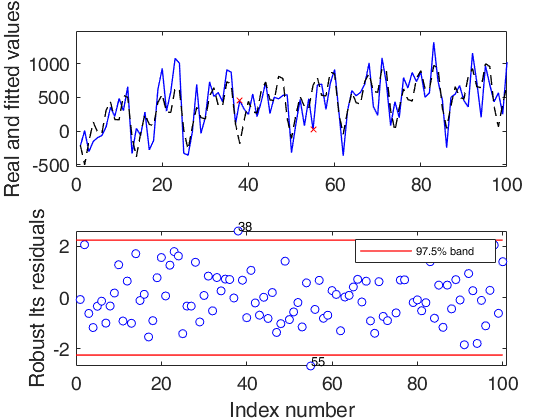
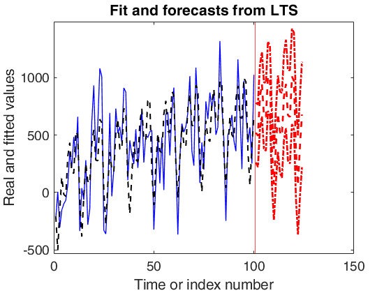
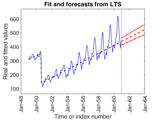
 Linear time varying seasonal component.
Linear time varying seasonal component.
close all
rng('default')
rng(1)
model=struct;
model.trend=1;
model.seasonal=103;
modelSIM=model;
modelSIM.trendb=[0 0];
modelSIM.seasonalb=40*[0.1 -0.5 0.2 -0.3 0.3 -0.1 0.222];
modelSIM.signal2noiseratio=20;
T=100;
% Simulate
outSIM=simulateTS(T,'model',modelSIM,'plots',1);
ySIM=outSIM.y;
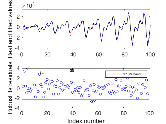
% Estimate
outEST=LTSts(ySIM,'model',model,'plots',1);
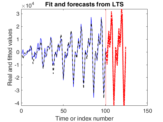
% Forecast
outFORE=forecastTS(outEST,'model',model,'plots',1);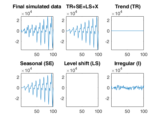
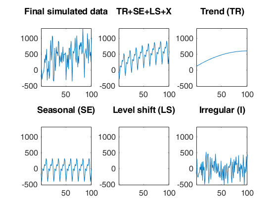
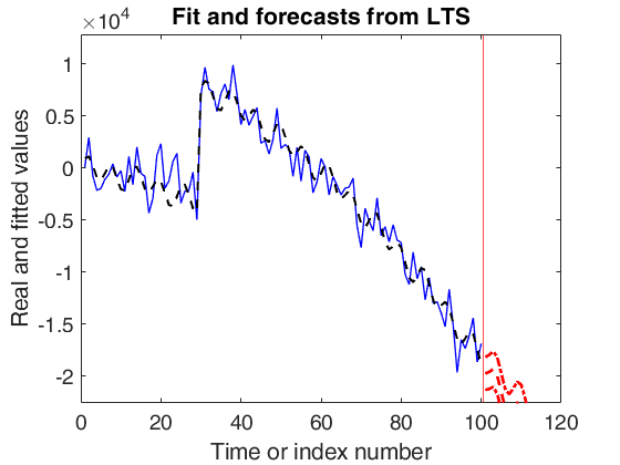
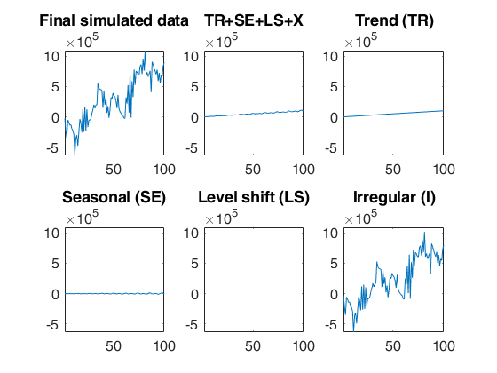
Quadratic trend and constant seasonal.
Quadratic trend and constant seasonal.
close all
rng(1)
model=struct;
model.trend=2;
model.seasonal=3;
modelSIM=model;
modelSIM.trendb=[100 10 -0.05];
modelSIM.seasonalb=400*[0.1 -0.5 0.2 -0.3 0.3 -0.1];
modelSIM.signal2noiseratio=1;
T=100;
% Simulate
outSIM=simulateTS(T,'model',modelSIM,'plots',1);
ySIM=outSIM.y;
% Estimate
outEST=LTSts(ySIM,'model',model,'plots',1);
% Forecast
outFORE=forecastTS(outEST,'model',model,'plots',1);
Related Examples
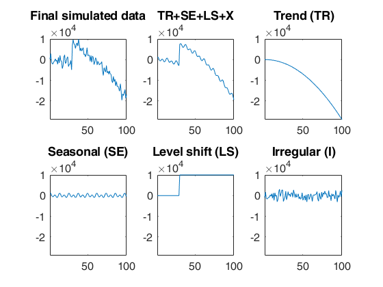
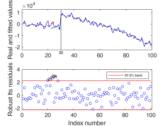
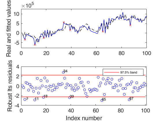
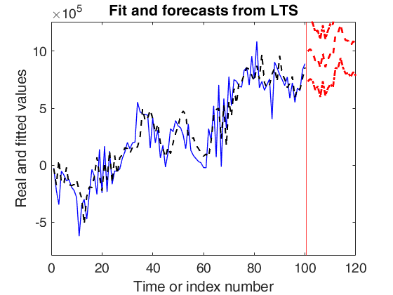
Simulated time series with quadratic trend, fixed seasonal and level shift.
Simulated time series with quadratic trend, fixed seasonal and level shift.A time series of 100 observations is simulated from a model which contains a quadratic trend, a seasonal component with two harmonics no explanatory variables and a level shift in position 30 with size 5000 and a signal to noise ratio equal to 20
close all
rng(1)
model=struct;
model.trend=2;
model.seasonal=2;
model.lshift=30;
modelSIM=model;
modelSIM.trendb=[5,10,-3];
modelSIM.seasonalb=100*[2 4 0.1 8];
modelSIM.signal2noiseratio=20;
modelSIM.lshiftb=10000;
T=100;
% Simulate
outSIM=simulateTS(T,'model',modelSIM,'plots',1);
ySIM=outSIM.y;
% Estimate
%  model.lshift=5:T-5 implies that LS is investigated from position
% $5, 6, 7, ..., T-5$,
model.lshift=5:T-5;
outEST=LTSts(ySIM,'model',model,'plots',1,'msg',0);
% Forecast
outFORE=forecastTS(outEST,'model',model,'plots',1);
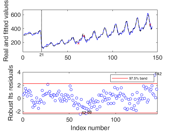
Contaminated airline data (1).
Contaminated airline data (1).Load the data.
%   1949 1950 1951 1952 1953 1954 1955 1956 1957 1958 1959 1960
y = [112  115  145  171  196  204  242  284  315  340  360  417   % Jan
118  126  150  180  196  188  233  277  301  318  342  391    % Feb
132  141  178  193  236  235  267  317  356  362  406  419    % Mar
129  135  163  181  235  227  269  313  348  348  396  461    % Apr
121  125  172  183  229  234  270  318  355  363  420  472    % May
135  149  178  218  243  264  315  374  422  435  472  535    % Jun
148  170  199  230  264  302  364  413  465  491  548  622    % Jul
148  170  199  242  272  293  347  405  467  505  559  606    % Aug
136  158  184  209  237  259  312  355  404  404  463  508    % Sep
119  133  162  191  211  229  274  306  347  359  407  461    % Oct
104  114  146  172  180  203  237  271  305  310  362  390    % Nov
118  140  166  194  201  229  278  306  336  337  405  432 ]; % Dec
y=y(:);
% Contaminate the first 20 observations
y(1:20)=y(1:20)+200;
close all
% Model with linear trend, three harmonics for seasonal component and
% varying amplitude using a linear trend. Search for a level shift
model=struct;
model.trend=1;              % linear trend
model.s=12;                 % monthly time series
model.seasonal=103;         % three harmonics with linear time varying seasonality
model.lshift=10:140;            % search for level shift
out=LTSts(y,'model',model,'plots',1,'dispresults',true,'msg',0);
% 3 years forecasts
nfore=36;
StartDate=[1949 1];
conflev=0.999; % Wide confidence level for the forecast
outFORE=forecastTS(out,'model',model,'nfore',nfore,'StartDate',StartDate,'conflev',conflev);
                  Coeff        SE          t           pval
                _________    _______    ________    ___________

    b_trend1        301.9     3.3707      89.565    1.9432e-121
    b_trend2       2.7697    0.03804      72.811    1.2536e-109
    b_cos1       -0.94446      2.822    -0.33468        0.73839
    b_sin1       -0.46559     1.3917    -0.33454         0.7385
    b_cos2      -0.036471    0.11546    -0.31586         0.7526
    b_sin2        0.55656     1.6636     0.33455        0.73849
    b_cos3        0.22205    0.66425     0.33428        0.73869
    b_sin3      -0.093486    0.28116     -0.3325        0.74003
    b_varaml      0.58107     1.7666     0.32891        0.74273
    b_lshift      -225.91     4.5415     -49.743     2.9417e-88

Level shift position t=21
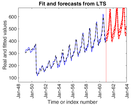
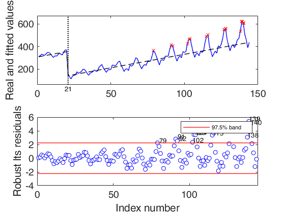
Contaminated airline data (2).
Contaminated airline data (2).
close all
% In this example we estimate a model without the seasonal component
%   1949 1950 1951 1952 1953 1954 1955 1956 1957 1958 1959 1960
y = [112  115  145  171  196  204  242  284  315  340  360  417   % Jan
118  126  150  180  196  188  233  277  301  318  342  391    % Feb
132  141  178  193  236  235  267  317  356  362  406  419    % Mar
129  135  163  181  235  227  269  313  348  348  396  461    % Apr
121  125  172  183  229  234  270  318  355  363  420  472    % May
135  149  178  218  243  264  315  374  422  435  472  535    % Jun
148  170  199  230  264  302  364  413  465  491  548  622    % Jul
148  170  199  242  272  293  347  405  467  505  559  606    % Aug
136  158  184  209  237  259  312  355  404  404  463  508    % Sep
119  133  162  191  211  229  274  306  347  359  407  461    % Oct
104  114  146  172  180  203  237  271  305  310  362  390    % Nov
118  140  166  194  201  229  278  306  336  337  405  432 ]; % Dec
y=y(:);
% Contaminate the first 20 observations
y(1:20)=y(1:20)+200;
% Model with linear trend and no seasonal component. Search for a level shift
model=struct;
model.trend=1;              % linear trend
model.s=12;                 % monthly time series
model.seasonal=0;          % no seasonal component
model.lshift=10:(length(y)-10);            % search for level shift
out=LTSts(y,'model',model,'plots',1,'dispresults',true,'msg',0);
% 3 years forecasts
nfore=36;
StartDate=[1949 1];
conflev=0.999; % Wide confidence level for the forecast
outFORE=forecastTS(out,'model',model,'nfore',nfore,'StartDate',StartDate,'conflev',conflev);
                 Coeff        SE          t          pval
                _______    ________    _______    __________

    b_trend1     307.43      7.2337       42.5    2.8696e-82
    b_trend2     2.3919    0.087445     27.354    3.0083e-58
    b_lshift    -214.71      9.7761    -21.963    2.3563e-47

Level shift position t=21
Forecast with autoregressive components and expl var.
Forecast with autoregressive components and expl var.Simulated data with linear trend, varying seasonal and AR(2)
rng(1000)
model=struct;
model.trend=1;
model.trendb=[5,1000];
model.seasonal=102;
model.seasonalb=100*[2 4 0.1 8 0.001];
model.signal2noiseratio=10;
model.ARp=[1 2];
model.ARb=[0.2 0.7];
model.ARIMAX=true;
T=100;
out=simulateTS(T,'model',model,'plots',1);
% Fit a model imposing linear trend, seasonal component and AR(2)
y=out.y;
nfore=20;
Xall=1e+2*randn(T+nfore,1);
X=Xall(1:T,:);
model=struct;
model.trend=1;
model.seasonal=102;
% No level shift
model.lshift=0;
% Add a non important expl. variable
model.X=X;
model.ARp=[1 2];
out=LTSts(y,'model',model,'plots',1,'dispresults',true);
% Note that in this case all the 120 values of Xall are supplied and
% the number of forecasts is 20
model.X=Xall;
forecastTS(out,'model',model,'nfore',20)
Iterative search of sigmaeps depending on the desired signal2noise ratio.
After 1000 iterations, the value of signal2noise ratio closest to the desired one is 10.0005,
obtained with sigmaeps = 107955.6243
                  Coeff         SE           t           pval
                _________    _________    ________    __________

    b_trend1       -16801        33939    -0.49503       0.62178
    b_trend2       2117.5       953.27      2.2214      0.028835
    b_cos1         -32427        21648     -1.4979       0.13766
    b_sin1          51362        27551      1.8642      0.065548
    b_cos2         6181.2        16773     0.36852       0.71335
    b_sin2         -39328        22569     -1.7426      0.084824
    b_auto 1      0.16847     0.064852      2.5978       0.01096
    b_auto 2      0.64325     0.065699      9.7907    7.7762e-16
    b_explX1       360.92       157.24      2.2954      0.024035
    b_varaml    0.0016604    0.0088853     0.18687       0.85218


ans =

  struct with fields:

          signal: [120×1 double]
           trend: [120×1 double]
        seasonal: [120×1 double]
               X: [100×10 double]
          lshift: 0
             XAR: 0
           Xexpl: [120×1 double]
        confband: [120×2 double]
    datesnumeric: [120×1 double]
Input Arguments
Output Arguments
References
Rousseeuw, P.J., Perrotta D., Riani M. and Hubert, M. (2018), Robust Monitoring of Many Time Series with Application to Fraud Detection, "Econometrics and Statistics". [RPRH]
See Also
LTSts
|
wedgeplot
|
simulateTS
|
LTStsVarSel