$N$ = $I$-by-$J$-contingency table. The $(i,j)$-th element is equal to
$n_{ij}$, $i=1, 2, \ldots, I$ and $j=1, 2, \ldots, J$. The sum of the
elements of N is $n$ (the grand total).
$P$=$I$-by-$J$-table containing correspondence matrix
(proportions). The $(i,j)$-th element is equal to
$n_{ij}/n$, $i=1, 2, \ldots, I$ and $j=1, 2,
\ldots, J$. The sum of the elements of $P$ is 1.
$P^*$=$I$-by-$J$-table containing correspondence matrix (proportions)
under the hypothesis of independence. The $(i,j)$-th element is equal to
$p_{ij}^*=p_{i.}p_{.j}$, $i=1, 2, \ldots, I$ and $j=1, 2, \ldots, J$.
The sum of the elements of $P^*$ is 1.
The power divergence family is defined:
\[
2n I^\lambda(P,P^*,\lambda) = \frac{2}{\lambda(\lambda+1)}
n \sum_{i=1}^{I} \sum_{j=1}^{J} p_{ij}
\left[ \left( \frac{p_{ij}}{p^*_{ij}} \right)^\lambda -1 \right]
\]
where $\lambda$ is the family parameter.
The term power divergence describes the fact that the statistic $2n
I^\lambda(P,P^*,\lambda)$ measures the divergence of $P$ from $P^*$
through a (weighted) sum of powers of the terms $\frac{p_{ij}}{p^*_{ij}}$
for $i=1, 2, \ldots, I$ and $j=1, 2, \ldots, J$.
The reference distribution (independently of the value of $\lambda$) is
$\chi^2$ with $(I-1) \times (J-1)$ degrees of freedom if (a) the hypothesis $H_0$ of
independence is true; (b) the sample size $n$ is large; (c) the number of
cells $I \times J$ is small relative to $n$ (and that all the expected cell
frequencies $n^*_{ij}$ are large); (d) unknown parameters are estimated with BAN
estimates; and (e) the models satisfy the regularity conditions of Birch
(1964) (Cressie and Read, 1984; p. 63).
If some of the expected frequencies are very small while others are
greater than 1, there are no firm recommendations regarding the best
approximation to use for the critical value. In some of these cases the
normal approximation may be appropriate, however the convergence of
this normal approximation is slow (Cressie and Read, 1984; p. 63).
The test we have just performed is intrinsically non-directional, that is
the significant value says nothing at all about the
particular direction of the difference.
Suggestions that X^2 approximates a chi-squared random variable more
closely than does G2 (for various multinomial and contingency table models)
have been made in enumeration and simulation studies.
Cressie and Read p. 85: extreme values of $\lambda$ are most useful for
detecting deviations from an expected cell frequency in a single cell
(i.e., bump or dip alternatives). Use of the maximum cell frequency to
test for "spikes" is discussed by Levin (1983); he also derives the
appropriate distributional results for hypothesis testing.
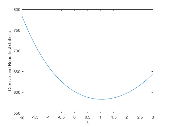
 Compute Cressie and Read statistic for a series of values of lambda.