FSRaddt

FSRaddt produces t deletion tests for each explanatory variable.

Syntax

Description

example

out =FSRaddt(y, X) FSRaddt with all default options.

example

out =FSRaddt(y, X, Name, Value) FSRaddt with optional arguments.

Examples

expand all

  • FSRaddt with all default options.
  • n=200;
    p=3;
    randn('state', 123456);
    X=randn(n,p);
    % Uncontaminated data
    y=randn(n,1);
    [out]=FSRaddt(y,X);

  • FSRaddt with optional arguments.
  • We perform a variable selection on the 'famous' stack loss data using different transformation scales for the response.

    load('stack_loss');
    y=stack_loss{:,4};
    X=stack_loss{:,1:3};
    %We start with a fan plot based on first-order model and the five most common values of $\lambda$ (Figure below).
    [out]=FSRfan(y,X,'plots',1);
    % The fan plot shows that the square root transformation, lambda= 0.5,
    % is supported by all the data, with the absolute value of the statistic
    % always less than 1.5. The evidence for all other transformations
    % depends on which observations have been deleted: the log transformation
    % is rejected when some of the suspected outliers are introduced into the
    % data although it is acceptable for all the data: ?= 1 is rejected as
    % soon as any of the suspected outliers are present.
    %
    % Given that the transformation for the response which is chosen
    % depends on the number of units declared as outliers we perform a
    % variable selection using the original scale, the square root and the
    % log transformation. 
    % Robust variable selection using original
    % untransformed values of the response
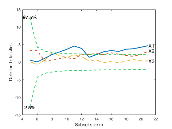
    % Monitoring of deletion t stat in the original scale
    [out]=FSRaddt(y,X,'plots',1,'quant',[0.025 0.975],'nsamp',5000);
    % Robust variable selection using square root values
    % Monitoring of deletion t stat using transformed response based on the square root
    [out]=FSRaddt(y.^0.5,X,'plots',1,'quant',[0.025 0.975]);
    % Robust variable selection using log transformed values of the response
    % Monitoring of deletion t stat using log transformed values
    [out]=FSRaddt(log(y),X,'plots',1,'quant',[0.025 0.975]);
    % Conclusion: the forward analysis based on the deletion t statistics
    % clearly reveals that variable X3, independently from the transformation
    % which is chosen and the number of outliers which are declared, is NOT
    % significant.
    Total estimated time to complete LMS:  0.00 seconds 
    Total estimated time to complete LMS:  0.00 seconds 
    Total estimated time to complete LMS:  0.00 seconds 
    Total estimated time to complete LMS:  0.00 seconds 
    Total estimated time to complete LMS:  0.00 seconds 
    Number of subsets to extract greater than (n p). It is set to (n p)
    Total estimated time to complete LMS:  0.01 seconds 
    Number of subsets to extract greater than (n p). It is set to (n p)
    Total estimated time to complete LMS:  0.00 seconds 
    Number of subsets to extract greater than (n p). It is set to (n p)
    Total estimated time to complete LMS:  0.15 seconds 
    ------------------------------
    Warning: Number of subsets without full rank equal to 14.1%
    Total estimated time to complete LMS:  0.00 seconds 
    Total estimated time to complete LMS:  0.00 seconds 
    Total estimated time to complete LMS:  0.00 seconds 
    ------------------------------
    Warning: Number of subsets without full rank equal to 14.4%
    Total estimated time to complete LMS:  0.00 seconds 
    Total estimated time to complete LMS:  0.00 seconds 
    Total estimated time to complete LMS:  0.01 seconds 
    ------------------------------
    Warning: Number of subsets without full rank equal to 14.1%
    
    Click here for the graphical output of this example (link to Ro.S.A. website).

    Related Examples

    expand all

  • FSRaddt with optional arguments.
  • Example of use of FSRaddt with plot of deletion t with personalized line width for the envelopes and personalized confidence interval.

    n=200;
    p=3;
    X=randn(n,p);
    y=randn(n,1);
    kk=9;
    y(1:kk)=y(1:kk)+6;
    X(1:kk,:)=X(1:kk,:)+3;
    [out]=FSRaddt(y,X,'plots',1,'quant',[0.025 0.975]);

  • FSRaddt with plots (transformed wool data).
  • load('wool');
    y=log(wool{:,end});
    X=wool{:,1:end-1};
    [out]=FSRaddt(y,X,'plots',1);

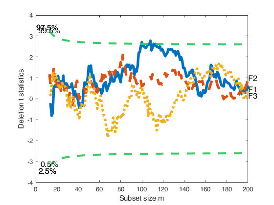
  • FSRaddt with labels for the columns of matrix X.
  • Line width equal to 3 for the curves representing envelopes; line width equal to 4 for the curves associated with deletion t stat.

    n=200;
    p=3;
    randn('state', 123456);
    X=randn(n,p);
    % Uncontaminated data
    y=randn(n,1);
    [out]=FSRaddt(y,X,'plots',1,'nameX',{'F1','F2','F3'},'lwdenv',3,'lwdt',4);
    Total estimated time to complete LMS:  0.01 seconds 
    Total estimated time to complete LMS:  0.01 seconds 
    Total estimated time to complete LMS:  0.01 seconds 
    
    Click here for the graphical output of this example (link to Ro.S.A. website)

    Input Arguments

    expand all

    y — Response variable. Vector.

    A vector with n elements that contains the response variable. It can be either a row or a column vector.

    Data Types: single| double

    X — Predictor variables. Matrix.

    Data matrix of explanatory variables (also called 'regressors') of dimension (n x p-1). Rows of X represent observations, and columns represent variables.

    Missing values (NaN's) and infinite values (Inf's) are allowed, since observations (rows) with missing or infinite values will automatically be excluded from the computations.

    Data Types: single| double

    Name-Value Pair Arguments

    Specify optional comma-separated pairs of Name,Value arguments. Name is the argument name and Value is the corresponding value. Name must appear inside single quotes (' '). You can specify several name and value pair arguments in any order as Name1,Value1,...,NameN,ValueN.

    Example: 'DataVars',[2 4] , 'intercept',false , 'h',round(n*0,75) , 'nsamp',1000 , 'lms',1 , 'init',100 starts monitoring from step m=100 , 'plots',1 , 'nameX',{'NameVar1','NameVar2'} , 'lwdenv',1 , 'msg',false , 'quant',[0.025 0.975] , 'lwdt',1 , 'nocheck',true , 'titl','Example' , 'labx','Subset' , 'laby','statistics' , 'FontSize',11 , 'SizeAxesNum',11 , 'ylimy',[0 1] , 'xlimy',[0 1]

    DataVars —Variables for which t deletion tests have to be computed.vector of positive integers | [].

    Columns of matrix X for which t deletion tests need to be computed. The default is empty, that is forward deletion t tests are computed for all the columns of matrix X.

    Example: 'DataVars',[2 4]

    Data Types: double

    intercept —Indicator for constant term.true (default) | false.

    Indicator for the constant term (intercept) in the fit, specified as the comma-separated pair consisting of 'Intercept' and either true to include or false to remove the constant term from the model.

    Example: 'intercept',false

    Data Types: boolean

    h —The number of observations that have determined the least trimmed squares estimator.scalar.

    h is an integer greater or equal than [(n+size(X,2)+1)/2] but smaller then n

    Example: 'h',round(n*0,75)

    Data Types: double

    nsamp —Number of subsamplse which will be extracted to find the robust estimator.scalar.

    If nsamp=0 all subsets will be extracted. They will be (n choose p). Remark: if the number of all possible subset is <1000 the default is to extract all subsets otherwise just 1000.

    Example: 'nsamp',1000

    Data Types: double

    lms —Criterion to use to find the initlal subset to initialize the search.scalar, vector | structure.

    If lms=1 (default) Least Median of Squares is computed, else Least Trimmed of Squares is computed. else (default) no plot is produced

    Example: 'lms',1

    Data Types: double

    init —Search initialization.scalar.

    Scalar which specifies the initial subset size to start monitoring exceedances of minimum deletion residual, if init is not specified it will be set equal to: p+1, if the sample size is smaller than 40;

    min(3*p+1,floor(0.5*(n+p+1))), otherwise.

    Example: 'init',100 starts monitoring from step m=100

    Data Types: double

    plots —Plot on the screen.scalar.

    If plots=1 a plot with forward deletion t-statistics is produced

    Example: 'plots',1

    Data Types: double

    nameX —Add variable labels in plot.cell array of strings.

    Cell array of strings of length p containing the labels of the varibles of the regression dataset. If it is empty (default) the sequence X1, ..., Xp will be created automatically

    Example: 'nameX',{'NameVar1','NameVar2'}

    Data Types: cell

    lwdenv —Line width for envelopes.scalar.

    Line width for envelopes based on student T (default is 2)

    Example: 'lwdenv',1

    Data Types: double

    msg —Level of output to display.boolean.

    It controls whether to display or not messages on the screen about subset size. If msg==true (default) messages are displayed on the screen about subset size every 100 steps, else no message is displayed on the screen.

    Example: 'msg',false

    Data Types: logical

    quant —Confidence quantiles for the envelopes.vector.

    Confidence quantiles for the envelopes of deletion t stat. Default is [0.005 0.995] (i.e. a 99 per cent pointwise confidence interval)

    Example: 'quant',[0.025 0.975]

    Data Types: double

    lwdt —Line width for deletion T stat.scalar.

    (default is 2)

    Example: 'lwdt',1

    Data Types: double

    nocheck —Check input arguments.boolean.

    If nocheck is equal to true no check is performed on matrix y and matrix X. Notice that y and X are left unchanged. In other words the additional column of ones for the intercept is not added. As default nocheck=false.

    Example: 'nocheck',true

    Data Types: boolean

    titl —a label for the title.character.

    (default: '')

    Example: 'titl','Example'

    Data Types: char

    labx —a label for the x-axis.character.

    (default: 'Subset size m')

    Example: 'labx','Subset'

    Data Types: char

    laby —a label for the y-axis.character.

    (default: 'Deletion t statistics')

    Example: 'laby','statistics'

    Data Types: char

    FontSize —the font size of the labels of the axes and of the labels inside the plot.scalar.

    Default value is 12

    Example: 'FontSize',11

    Data Types: double

    SizeAxesNum —size of the numbers of the axes.scalar.

    Default value is 10

    Example: 'SizeAxesNum',11

    Data Types: double

    ylimy —minimum and maximum of the y axis.vector.

    Default value is '' (automatic scale)

    Example: 'ylimy',[0 1]

    Data Types: double

    xlimx —minimum and maximum of the x axis.vector.

    Default value is '' (automatic scale)

    Example: 'xlimy',[0 1]

    Data Types: double

    Output Arguments

    expand all

    out — description Structure

    Structure which contains the following fields

    Value Description
    Tdel

    (n-init+1) x (p+1) matrix containing the monitoring of deletion t stat in each step of the forward search 1st col = fwd search index (from init to n) 2nd col = deletion t stat for first explanatory variable 3rd col = deletion t stat for second explanatory variable ...

    (p+1)th col = deletion t stat for pth explanatory variable

    S2del

    (n-init+1) x (p+1) matrix containing the monitoring of deletion S2 stat in each step of the forward search 1st col = fwd search index (from init to n) 2nd col = estimate of $\sigma^2$ when the ordering of the units to enter the fwd search is found excluding first explanatory variable 3rd col = estimate of $\sigma^2$ when the ordering of the units to enter the fwd search is found excluding second explanatory variable ...

    (p+1)th col = estimate of $\sigma^2$ when the ordering of the units to enter the fwd search is found excluding last explanatory variable

    bs

    matrix of size p x length(DataVars) containing the units forming the initial subset of length p for the searches associated with the deletion t statistics.

    Un

    cell of length length(DataVars).

    out.Un{i} (i=1, ..., ength(DataVars)) is a (n-init) x 11 matrix which contains the unit(s) included in the subset at each step in the search which excludes the ith explanatory variable.

    REMARK: in every step the new subset is compared with the old subset. Un contains the unit(s) present in the new subset but not in the old one Un(1,:) for example contains the unit included in step init+1 ... Un(end,2) contains the units included in the final step of the search

    y

    A vector with n elements that contains the response variable which has been used

    X

    Data matrix of explanatory variables which has been used (it also contains the column of ones if input option intercept was missing or equal to 1)

    la

    Vector containing the numbers associated to matrix out.X for which deletion t stat have been computed. For example is the intercept is present and input option DataVars was equal to [1 3], out.la=[2 4].

    class

    'FSRaddt';

    References

    Atkinson, A.C. and Riani, M. (2002b), Forward search added variable t tests and the effect of masked outliers on model selection, "Biometrika", Vol. 89, pp. 939-946.

    See Also

    This page has been automatically generated by our routine publishFS