MixSimreg
MixSimreg generates k regression hyperplanes in p dimensions with given overlap
Description
MixSimreg(k,p) generates k groups in p dimensions. It is possible to control the average and maximum or standard deviation of overlapping.
Notation and background.
Given two generic clusters $i$ and $j$ with $i \ne j=1,...,k$, indexed by $\phi(x,\mu_i,\sigma_i^2)$ and $\phi(x,\mu_j, \sigma_j^2)$ with probabilities of occurrence $\pi_i$ and $\pi_j$, the misclassification probability with respect to cluster $i$ (denoted with $w_{j|i}$) is defined as
\[ Pr[\pi_i \phi(x,\mu_i,\sigma_i^2) < \pi_j \phi(x,\mu_j,\sigma_j^2)] \]where, in the regression context, $\mu_i={\overline x}_i' \beta_i$ and $\mu_j= \overline x_j' \beta_j$. We assume that the length of vectors $x_i$, $x_j$, $\beta_i$, and $\beta_j$ is $p$ (number of explanatory variables including or excluding intercept). In our implementation, the distribution of the elements of vectors $\beta_i$ ($\beta_j$) can be 'Normal' (with parameters $\mu$ and $\sigma$), 'HalfNormal' (with parameter $\sigma$) or uniform (with parameters $a$ and $b$). Same thing for the distribution of the elements of $x_i$ ($x_j$). However, while the parameters of the distributions are the same for all elements of $\beta$ in all groups, the parameters of the distribution of the elements of vectors $x_i$ ($x_j$) can vary for each group and each explanatory variable. In other words, it is possible to specify (say) that the distribution of the second explanatory variable in the first group is $U(2, 3)$ while the distribution of the third explanatory variable in the second group is $U(2, 10)$.
The matrix containing the misclassification probabilities $w_{j|i}$ is called OmegaMap.
The probability of overlapping between groups i and j is given by
\[ w_{j|i} + w_{i|j} \qquad i,j=1,2, ..., k \]The diagonal elements of OmegaMap are equal to 1.
The average overlap (BarOmega, in the code) is defined as the sum of the off diagonal elements of OmegaMap (containing the misclassification probabilities) divided by $k*(k-1)/2$.
The maximum overlap (MaxOmega, in the code) is defined as:
\[ \max (w_{j|i} + w_{i|j}) \qquad i \ne j=1,2, ..., k \]The probability of overlapping $w_{j|i}$ is nothing but the cdf of a linear combination of non central $\chi^2$ distributions with 1 degree of freedom plus a linear combination of $N(0,1)$ evaluated in a point $c$.
The coefficients of the linear combinations of non central $\chi^2$ and $N(0,1)$ and point c depend on $\sigma_{j|i}^2 = \sigma_i^2/\sigma_j^2$.
This probability is computed using routine ncx2mixtcdf
Example 2: Mixture of regression with prefixed average overlap.out
=MixSimreg(k,
p,
Name, Value)
Examples
 Example 1: Mixture of regression with prefixed average overlap.
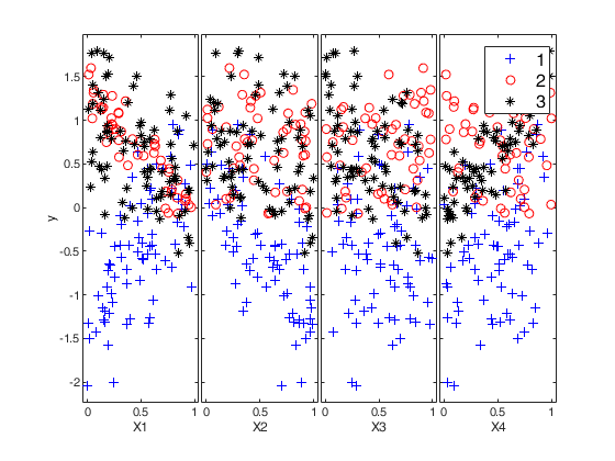
Example 1: Mixture of regression with prefixed average overlap.Generate mixture of regression using an average overlapping at centroids =0.01. Use all default options 1) Beta is generated according to random normal for each group with mu=0 and sigma=1 2) X in each dimension and each group is generated according to U(0, 1) 3) regression hyperplanes contain intercepts
p=5;
k=3;
out=MixSimreg(k,p,'BarOmega',0.01);
n=200;
% out.Xdistrib.BarX in this case has dimension 5-by-3 and is equal to
% 1.0000    1.0000    1.0000
% 0.5000    0.5000    0.5000
% 0.5000    0.5000    0.5000
% 0.5000    0.5000    0.5000
% 0.5000    0.5000    0.5000
% Probabilities of overlapping are evaluated at
% out.Beta(:,1)'*out.Xdistrib.BarX(:,1) ... out.Beta(:,3)'*out.Xdistrib.BarX(:,3)
[y,X,id]=simdatasetreg(n,out.Pi,out.Beta,out.S,out.Xdistrib);
yXplot(y,X(:,2:end),'group',id);
Related Examples
Example 8: Another Tweedie-based international trade data example.
Example 8: Another Tweedie-based international trade data example.This is like example 7, but with group-specific Tweedie distributions.
n=500;
p=1;
k=3;
% generate three Tweedie distributed explanatory variables
[alpha,theta,delta] = deal(0.5 , 5 , 1);
alpha2 = 0.7;
alpha3 = 0.9;
X1 = twdrnd(alpha,theta,delta,floor(n/3));
X2 = twdrnd(alpha2,theta,delta,floor(n/3));
X3 = twdrnd(alpha3,theta,delta,n-2*floor(n/3));
% Distribution of the explanatory variable: the mean the three Tweedie
% components is specified
Xdistrib=struct;
Xdistrib.intercept=0;
Xdistrib.type='User';
Xdistrib.BarX = [mean(X1) , mean(X2) , mean(X3)];
% Distribution of the regression parameters
betadistrib=struct;
betadistrib.type='HalfNormal';
betadistrib.sigma=6;
% Overlap level: BarOmega=0.1
close all
rng(10,'twister')
Q=MixSimreg(k,p,'BarOmega',0.1,'Xdistrib',Xdistrib,'betadistrib',betadistrib);
% The three X-components
Q.Xdistrib.X = [X1 ; X2 ; X3];
% Now simulate the dataset
[y,X,id]=simdatasetreg(n,Q.Pi,Q.Beta,Q.S,Q.Xdistrib);
% And plot it
yXplot(y,X,'group',id,'tag','Strong_Overlap');
set(gcf,'Name','explanatory variable is Tweedie distributed');
title('Three components with different Tweedie-distributed explanatory variables');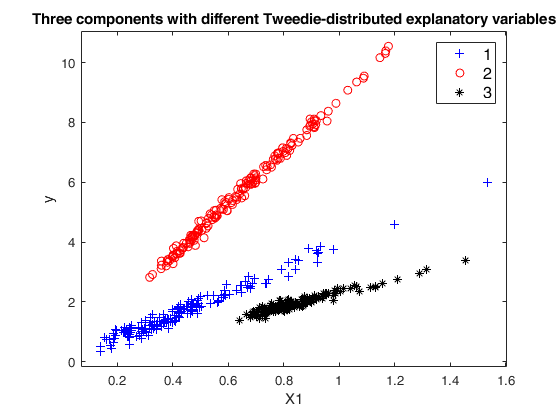
Input Arguments
Output Arguments
References
Maitra, R. and Melnykov, V. (2010), Simulating data to study performance of finite mixture modeling and clustering algorithms, "The Journal of Computational and Graphical Statistics", Vol. 19, pp. 354-376. [to refer to this publication we will use "MM2010 JCGS"]
Melnykov, V., Chen, W.-C. and Maitra, R. (2012), MixSim: An R Package for Simulating Data to Study Performance of Clustering Algorithms, "Journal of Statistical Software", Vol. 51, pp. 1-25.
Davies, R. (1980), The distribution of a linear combination of chi-square random variables, "Applied Statistics", Vol. 29, pp. 323-333.
Parlett, B.N. and Reinsch, C. (1969), Balancing a matrix for calculation of eigenvalues and eigenvectors, "Numerische Mathematik", Vol. 13, pp. 293-304.
Parlett, B.N. and Reinsch, C. (1971), Balancing a Matrix for Calculation of Eigenvalues and Eigenvectors, in Bauer, F.L. Eds, "Handbook for Automatic Computation", Vol. 2, pp. 315-326, Springer.
Garcia-Escudero, L.A., Gordaliza, A., Matran, C. and Mayo-Iscar, A. (2008), A General Trimming Approach to Robust Cluster Analysis. Annals of Statistics, Vol. 36, 1324-1345.
Torti F., Perrotta D., Riani, M. and Cerioli A. (2019). Assessing Robust Methodologies for Clustering Linear Regression Data, "Advances in Data Analysis and Classification", Vol. 13, pp. 227–257, https://doi.org/10.1007/s11634-018-0331-4
See Also
tkmeans
|
tclust
|
tclustreg
|
lga
|
rlga
|
ncx2mixtcdf
|
restreigen