FM_spot_vol
FM_spot_vol computes the spot volatility of a diffusion process via the Fourier-Malliavin estimator
Syntax
Description
Examples
 Example of call of FM_spot_vol with default values of M,N and tau.
Example of call of FM_spot_vol with default values of M,N and tau.The following example estimates the path of the spot volatility of a Heston model from a discrete sample. The Heston model assumes that the spot variance follows a Cox-Ingersoll-Ross model.
% Heston model simulation
T=1;
n=23400;
parameters=[0,0.4,2,1];
Rho=-0.5;
x0=log(100);
V0=0.4;
[x,V,t]=Heston1D(T,n,parameters,Rho,x0,V0);
% Spot volatility estimation
[V_spot, tau_out]=FM_spot_vol(x,t,T);
M=(length(V_spot)-1)/2;
figure
plot(tau_out,V(1:round(n/(2*M)):end));
hold on
plot(tau_out,V_spot);
xlabel('tau');
title('Spot volatility estimates Vs Actual values')
legend('Actual values','Estimated values')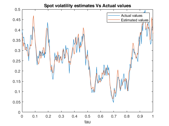
Example of call of FM_spot_vol with custom choices of M,N and tau.
Example of call of FM_spot_vol with custom choices of M,N and tau.The following example estimates the path of the spot volatility of a Heston model from a discrete sample. The Heston model assumes that the spot variance follows a Cox-Ingersoll-Ross model.
% Heston model simulation
T=1;
n=23400;
parameters=[0,0.4,2,1];
Rho=-0.5;
x0=log(100);
V0=0.4;
[x,V,t]=Heston1D(T,n,parameters,Rho,x0,V0);
% Spot volatility estimation
tau=0:T/50:T;
[V_spot, tau_out]= FM_spot_vol(x,t,T,'N',5000,'M',100,'tau',tau);
figure
plot(tau_out,V(1:round(n/50):end));
hold on
plot(tau_out,V_spot);
xlabel('tau');
title('Spot volatility estimates Vs Actual values')
legend('Actual values','Estimated values')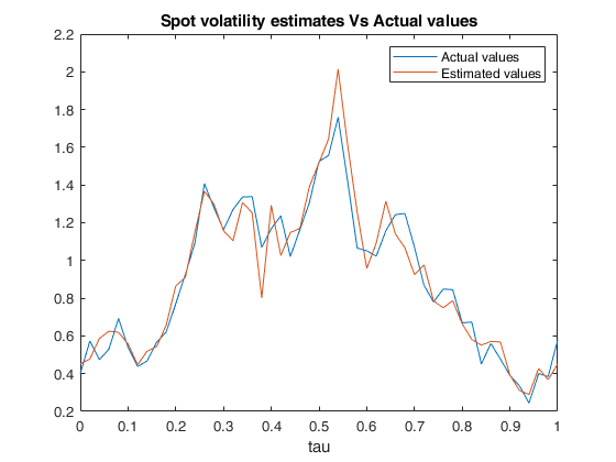
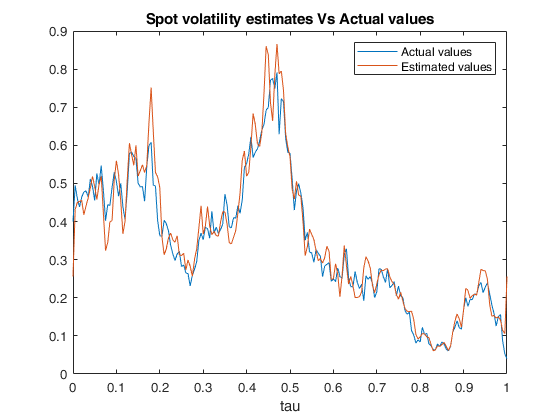
Example of call of FM_spot_vol when tau has length larger than 2M + 1.
Example of call of FM_spot_vol when tau has length larger than 2M + 1.The following example estimates the path of the spot volatility of a Heston model from a discrete sample. The Heston model assumes that the spot variance follows a Cox-Ingersoll-Ross model.
% Heston model simulation
T=1;
n=23400;
parameters=[0,0.4,2,1];
Rho=-0.5;
x0=log(100);
V0=0.4;
[x,V,t]=Heston1D(T,n,parameters,Rho,x0,V0);
% Spot volatility estimation
tau=0:T/1000:T;
[V_spot, tau_out]= FM_spot_vol(x,t,T,'N',5000,'M',100,'tau',tau);
figure
M=100;
plot(tau_out,V(1:round(n/(2*M)):end));
hold on
plot(tau_out,V_spot);
xlabel('tau');
title('Spot volatility estimates Vs Actual values')
legend('Actual values','Estimated values')
WARNING: estimation will be performed on the equally-spaced grid with mesh size equal to T/(2*M), provided as an output variable.
Input Arguments
Output Arguments
More About
References
Mancino, M.E., Recchioni, M.C., Sanfelici, S. (2017), Fourier-Malliavin Volatility Estimation. Theory and Practice, "Springer Briefs in Quantitative Finance", Springer.
Sanfelici, S., Toscano, G. (2024), The Fourier-Malliavin Volatility (FMVol) MATLAB toolbox, available on ArXiv.
See Also
FE_spot_vol
|
FE_spot_vol_FFT
|
FM_spot_quart
|
FM_spot_volvol
|
FM_spot_lev
|
Heston1D