Sregeda
Sregeda computes S estimators in linear regression for a series of values of bdp
Syntax
Description
Examples
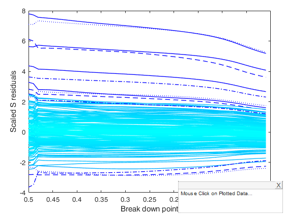
 Sregeda with msg=0.
Sregeda with msg=0.Run this code to see the output shown in the help file.
n=200;
p=3;
randn('state', 123456);
X=randn(n,p);
% Uncontaminated data
y=randn(n,1);
% Contaminated data
ycont=y;
ycont(1:5)=ycont(1:5)+6;
[out]=Sregeda(ycont,X,'msg',0);
resfwdplot(out)
ylabel('Scaled S residuals');
Related Examples
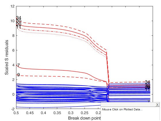
Sreg on Stars data.
Sreg on Stars data.Run this code to see the Figure 2 of the article in the References.
load('stars');
X=stars{:,1};
y=stars{:,2};
[out]=Sregeda(y,X,'rhofunc','bisquare');
standard.Color={'b'}
standard.xvalues=size(out.RES,1)-size(out.RES,2)+1:size(out.RES,1)
fground.Color={'r'}
resfwdplot(out,'standard',standard,'fground',fground)
ylabel('Scaled S residuals');
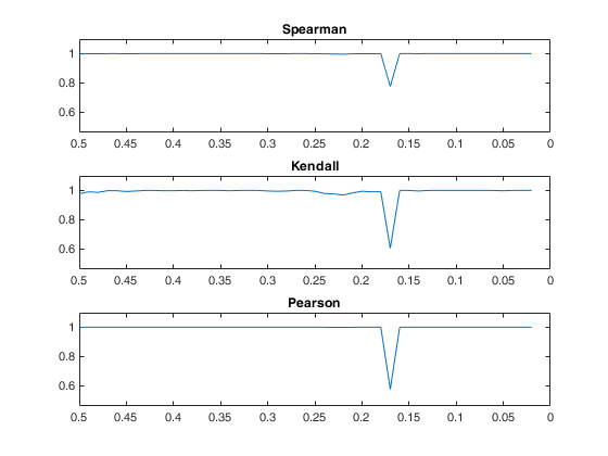
RHO = [];
for i=1:49
RHO(i,1) = corr(out.RES(:,i),out.RES(:,i+1),'type','Spearman');
RHO(i,2) = corr(out.RES(:,i),out.RES(:,i+1),'type','Kendall');
RHO(i,3) = corr(out.RES(:,i),out.RES(:,i+1),'type','Pearson');
end
minc = min(RHO);
maxc = max(RHO);
ylimits = [min(minc)*0.8,max(maxc)*1.1];
figure;
subplot(3,1,1);
plot(out.bdp(1:49),RHO(:,1)');
if strcmp(out.class,'Sregeda')
set(gca,'XDir','reverse','ylim',ylimits);
title('Spearman');
end
subplot(3,1,2);
plot(out.bdp(1:49),RHO(:,2)');
if strcmp(out.class,'Sregeda')
set(gca,'XDir','reverse','ylim',ylimits);
title('Kendall');
end
subplot(3,1,3);
plot(out.bdp(1:49),RHO(:,3)');
if strcmp(out.class,'Sregeda')
set(gca,'XDir','reverse','ylim',ylimits);
title('Pearson');
end
Total estimated time to complete S estimate:  0.56 seconds
Total estimated time to complete S estimate:  0.51 seconds
Total estimated time to complete S estimate:  0.19 seconds
Total estimated time to complete S estimate:  0.18 seconds
Total estimated time to complete S estimate:  0.18 seconds
Total estimated time to complete S estimate:  0.19 seconds
Total estimated time to complete S estimate:  0.18 seconds
Total estimated time to complete S estimate:  0.17 seconds
Total estimated time to complete S estimate:  0.17 seconds
Total estimated time to complete S estimate:  0.17 seconds
Total estimated time to complete S estimate:  0.17 seconds
Total estimated time to complete S estimate:  0.17 seconds
Total estimated time to complete S estimate:  0.16 seconds
Total estimated time to complete S estimate:  0.17 seconds
Total estimated time to complete S estimate:  0.18 seconds
Total estimated time to complete S estimate:  0.16 seconds
Total estimated time to complete S estimate:  0.19 seconds
Total estimated time to complete S estimate:  0.15 seconds
Total estimated time to complete S estimate:  0.16 seconds
Total estimated time to complete S estimate:  0.15 seconds
Total estimated time to complete S estimate:  0.16 seconds
Total estimated time to complete S estimate:  0.15 seconds
Total estimated time to complete S estimate:  0.16 seconds
Total estimated time to complete S estimate:  0.32 seconds
Total estimated time to complete S estimate:  0.15 seconds
Total estimated time to complete S estimate:  0.15 seconds
Total estimated time to complete S estimate:  0.15 seconds
Total estimated time to complete S estimate:  0.17 seconds
Total estimated time to complete S estimate:  0.23 seconds
Total estimated time to complete S estimate:  0.24 seconds
Total estimated time to complete S estimate:  0.18 seconds
Total estimated time to complete S estimate:  0.20 seconds
Total estimated time to complete S estimate:  0.14 seconds
Total estimated time to complete S estimate:  0.17 seconds
Total estimated time to complete S estimate:  0.11 seconds
Total estimated time to complete S estimate:  0.12 seconds
Total estimated time to complete S estimate:  0.10 seconds
Total estimated time to complete S estimate:  0.10 seconds
Total estimated time to complete S estimate:  0.09 seconds
Total estimated time to complete S estimate:  0.13 seconds
Total estimated time to complete S estimate:  0.10 seconds
Total estimated time to complete S estimate:  0.09 seconds
Total estimated time to complete S estimate:  0.08 seconds
Total estimated time to complete S estimate:  0.08 seconds
Total estimated time to complete S estimate:  0.09 seconds
Total estimated time to complete S estimate:  0.10 seconds
Total estimated time to complete S estimate:  0.08 seconds
Total estimated time to complete S estimate:  0.08 seconds
Total estimated time to complete S estimate:  0.09 seconds
Total estimated time to complete S estimate:  0.08 seconds

standard =

  struct with fields:

    Color: {'b'}


standard =

  struct with fields:

      Color: {'b'}
    xvalues: [-2 -1 0 1 2 3 4 5 6 7 8 9 10 11 12 13 14 15 16 … ] (1×50 double)


fground =

  struct with fields:

    Color: {'r'}
Input Arguments
Output Arguments
References
Riani, M., Cerioli, A., Atkinson, A.C. and Perrotta, D. (2014), Monitoring Robust Regression, "Electronic Journal of Statistics", Vol. 8, pp. 646-677.
Maronna, R.A., Martin D. and Yohai V.J. (2006), "Robust Statistics, Theory and Methods", Wiley, New York.