smothr
smothr produces smoothed values with constraints.
Description
This function is used in each step of the iterative procedure for ACE, but can be called directly when it is necessary to smooth a set of values. Note that the x values must be non decreasing.
Examples
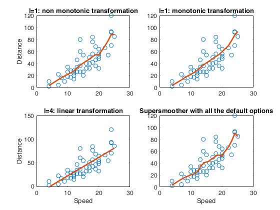
 Compare 4 different smoothers.
Compare 4 different smoothers.The data give the speed of cars and the distances taken to stop. Note that the data were recorded in the 1920s.
% The first column of X is speed, while the second is the time to stop.
X=[ 4    2
4   10
7    4
7   22
8   16
9   10
10   18
10   26
10   34
11   17
11   28
12   14
12   20
12   24
12   28
13   26
13   34
13   34
13   46
14   26
14   36
14   60
14   80
15   20
15   26
15   54
16   32
16   40
17   32
17   40
17   50
18   42
18   56
18   76
18   84
19   36
19   46
19   68
20   32
20   48
20   52
20   56
20   64
22   66
23   54
24   70
24   92
24   93
24  120
25   85];
x=X(:,1);
y=X(:,2);
% Compare the output.
subplot(2,2,1)
% Non monotonic output l=1.
plot(x,y,'o')
hold('on')
l=1;
ysmo=smothr(l,x,y);
plot(x,ysmo,'-','LineWidth',2)
title('l=1: non monotonic transformation')
ylabel('Distance')
subplot(2,2,2)
% Impose monotonic output.
% Input option l=3.
plot(x,y,'o')
hold('on')
l=3;
ysmo=smothr(l,x,y);
plot(x,ysmo,'-','LineWidth',2)
title('l=1: monotonic transformation')
subplot(2,2,3)
% Impose monotonic output.
% Input option l=4.
plot(x,y,'o')
hold('on')
l=4;
% Impose a linear smoother
ysmo=smothr(l,x,y);
plot(x,ysmo,'-','LineWidth',2)
title('l=4: linear transformation')
xlabel('Speed')
ylabel('Distance')
subplot(2,2,4)
% Impose monotonic output
plot(x,y,'o')
hold('on')
ysmo=supsmu(x,y);
plot(x,ysmo,'-','LineWidth',2)
title('Supersmoother with all the default options')
xlabel('Speed')
ylabel('Distance')
Input Arguments
Output Arguments
References
Breiman, L. and Friedman, J.H. (1985), Estimating optimal transformations for multiple regression and correlation, "Journal of the American Statistical Association", Vol. 80, pp. 580-597.
Wang D. and Murphy M. (2005), Identifying nonlinear relationships regression using the ACE algorithm, "Journal of Applied Statistics", Vol. 32, pp. 243-258.
Friedman, J.H. (1984), A variable span scatterplot smoother. Laboratory for Computational Statistics, Stanford University, Technical Report No. 5.